Mathematics · Ch 7 — Linear Programming
Graphical representation of linear inequations in two variables
Graphical representation of linear inequations in two variables
This sub-section fixes the standard shading convention for four increasingly general families of linear inequation in two
variables, each illustrated with a small reference graph.
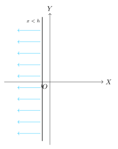
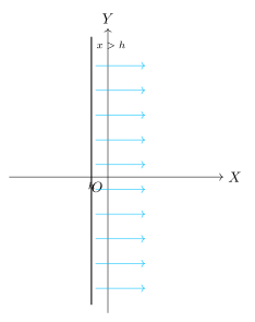
1) and . Draw the vertical line in the plane. Every point to the LEFT of this line has an
-coordinate smaller than , so the solution set of is the closed half-plane on and to the left of the line;
correspondingly, the solution set of is the closed half-plane on and to the right of the line.
Drawn by us to help you understand the concept clearly, and verified to make sure it's accurate. For exams, practice from your textbook's own diagram.
fig 7.4 — solution of x ≤ h: the half-plane on and to the left of the vertic …
Drawn by us to help you understand the concept clearly, and verified to make sure it's accurate. For exams, practice from your textbook's own diagram.
fig 7.5 — solution of x ≥ h: the half-plane on and to the righ …
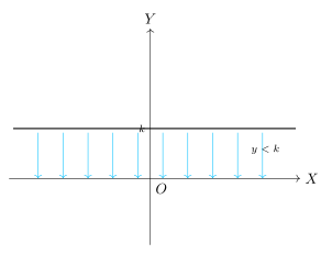
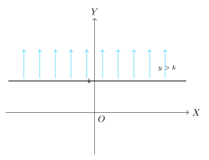
2) and . Draw the horizontal line . The solution set of is the closed half-plane on and
below this line, and the solution set of is the closed half-plane on and above it.
Drawn by us to help you understand the concept clearly, and verified to make sure it's accurate. For exams, practice from your textbook's own diagram.
fig 7.6 — solution of y ≤ k: the half-plane on and below the horizonta …
Drawn by us to help you understand the concept clearly, and verified to make sure it's accurate. For exams, practice from your textbook's own diagram.
fig 7.7 — solution of y ≥ k: the half-plane on and ab …
3) and (line through the origin). When the line passes through the origin (no
constant term), the origin lies exactly ON the boundary and so cannot be used to test which side is which — a different
point not on the line must be substituted instead, and the half-plane containing that test point is shaded according to
whichever inequality it satisfies.
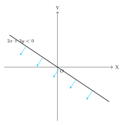
Drawn by us to help you understand the concept clearly, and verified to make sure it's accurate. For exams, practice from your textbook's own diagram.
fig 7.8 — solution of 2x + 3y ≤ 0: a half-plane bounded by a line throug …
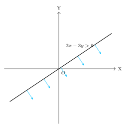
Drawn by us to help you understand the concept clearly, and verified to make sure it's accurate. For exams, practice from your textbook's own diagram.
fig 7.9 — solution of 2x − 3y ≥ 0: a half-plane bounded by a line throug …
4) and (general line, using the origin as test point). Draw the line ; this line
divides the plane into two half-planes, conventionally labelled , the "origin side" of the line (the half-plane
containing the point ), and , the "non-origin side" (the other half-plane). Substitute the origin's
coordinates into the given inequation: if satisfies , then the required region is the origin side
, and should be shaded; otherwise, the required region is the non-origin side . The points where …
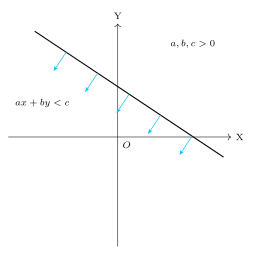
Drawn by us to help you understand the concept clearly, and verified to make sure it's accurate. For exams, practice from your textbook's own diagram.
fig 7.10 — solution of ax + by ≤ c (a,b,c>0): the origin side H₁ of the lin …
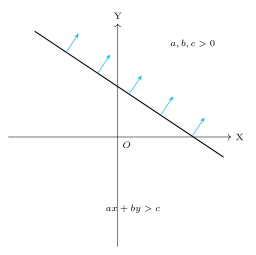
Drawn by us to help you understand the concept clearly, and verified to make sure it's accurate. For exams, practice from your textbook's own diagram.
fig 7.11 — solution of ax + by ≥ c (a,b,c>0): the non-origin side H₂ of the lin …