Mathematics · Ch 7 — Linear Programming
Graphical solution of linear inequation
Graphical solution of linear inequation
This sub-section works through six fully solved examples applying the shading method of section 7.1.2.
Example 1 — six single inequations, each solved by finding the boundary line and testing a point.
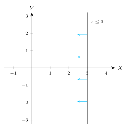
a) : the boundary is the vertical line . The origin gives , true, so the origin side (the
region to the LEFT of , including the line) is shaded.
Drawn by us to help you understand the concept clearly, and verified to make sure it's accurate. For exams, practice from your textbook's own diagram.
fig 7.12 — solution set of x ≤ 3 (origin side o …
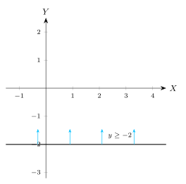
b) : the boundary is the horizontal line . The origin gives , true, so the origin side (the region
ABOVE , including the line) is shaded.
Drawn by us to help you understand the concept clearly, and verified to make sure it's accurate. For exams, practice from your textbook's own diagram.
fig 7.13 — solution set of y ≥ −2 (origin side of …
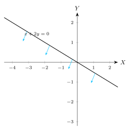
c) : rewritten as , this line passes through the origin, so the origin cannot serve as the test point.
Choosing instead: , and is true, so the half-plane containing is
shaded.
Drawn by us to help you understand the concept clearly, and verified to make sure it's accurate. For exams, practice from your textbook's own diagram.
fig 7.14 — solution set of x + 2y ≤ 0 (boundary line through t …
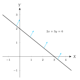
d) : the boundary line passes through and (its intercepts). Testing the origin:
, and is FALSE, so the origin side is excluded — the required region is the NON-origin side of the
line.
Drawn by us to help you understand the concept clearly, and verified to make sure it's accurate. For exams, practice from your textbook's own diagram.
fig 7.15 — solution set of 2x + 3y ≥ 6 (non-orig …
e) : the boundary line passes through and . Testing the origin: , and
is TRUE, so the required region IS the origin side of the line.
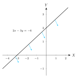
Drawn by us to help you understand the concept clearly, and verified to make sure it's accurate. For exams, practice from your textbook's own diagram.
fig 7.16 — solution set of 2x − 3y ≥ −6 (orig …
f) : the boundary line passes through and . Testing the origin: , and
is TRUE, so the required region is the origin side of the line.
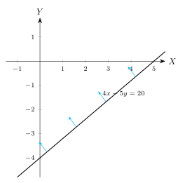
Drawn by us to help you understand the concept clearly, and verified to make sure it's accurate. For exams, practice from your textbook's own diagram.
fig 7.17 — solution set of 4x − 5y ≤ 20 (orig …
Example 2 — . Draw the line through its intercepts and . Testing the origin:
, true — the origin side of the line is the required region.
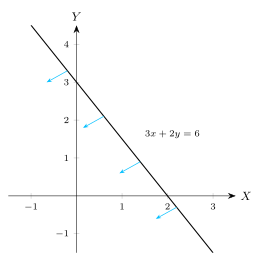
Drawn by us to help you understand the concept clearly, and verified to make sure it's accurate. For exams, practice from your textbook's own diagram.
fig 7.18 — solution set of 3x + 2y ≤ 6 (origi …
Example 3 — the system and . Draw both boundary lines: through and , and
through and . Testing the origin in each: for , gives , FALSE, so this
constraint's shaded region is the NON-origin side; for , gives , TRUE, so this constraint's
shaded region is the origin side. The common (overlapping) region of these two oppositely-labelled half-planes is the
graphical solution of the system — an unbounded region (since neither inequation caps the plane on every side), whose
single corner point is found by solving and simultaneously: from the second equation ;
substituting into the first, . So the
corner point is .
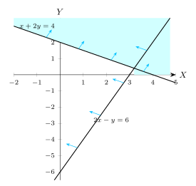
Drawn by us to help you understand the concept clearly, and verified to make sure it's accurate. For exams, practice from your textbook's own diagram.
fig 7.19 — common region of x + 2y ≥ 4 and 2x − y ≤ 6 (unbounded; corner …
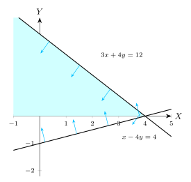
Example 4 — the system and . Draw both lines: through and , and
through and (note both lines happen to pass through the same point ). Testing the
origin in each gives (true) and (true, in fact strictly), so BOTH constraints shade their origin
side, and the common shaded region — the graphical solution — is the overlap of the two origin-side half-planes, an
unbounded wedge-shaped region with its one finite corner at the shared point where the two lines cross.
Drawn by us to help you understand the concept clearly, and verified to make sure it's accurate. For exams, practice from your textbook's own diagram.
fig 7.20 — common region of 3x + 4y ≤ 12 and x − 4y ≤ 4 (unbounded wedge; c …
Note on plotting a line via the double-intercept form. As an alternative to picking two arbitrary points, any line
(with ) can be written in double-intercept form by dividing through by : for example
becomes , immediately showing the -intercept is and the -intercept is , i.e. the
line passes through and — the same two points used to draw it above.
Feasible solutions of a system of inequations (introducing the term). When several linear inequations must hold at the same time — together with the non-negativity constraints — the region common to all of them is called the feasible region, and every point of it is a feasible solution. The same origin-side / non-origin-side shading method of section 7.1.2 is applied to each constraint, and the overlap of all the shaded half-planes is the feasible region.
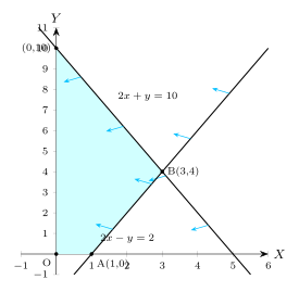
Example 1. Find the graphical solution of the system . Draw (through and ) and (through and ); testing the origin, each constraint shades its origin side, and within the first quadrant the common shaded region is a bounded quadrilateral with vertices , , and . This common shaded region is the feasible solution of the system.
Drawn by us to help you understand the concept clearly, and verified to make sure it's accurate. For exams, practice from your textbook's own diagram.
fig 7.21 — feasible region OABCO of 2x + y ≤ 10, 2x − y ≤ 2, x,y ≥ 0; vertices O, A(1,0), …
…
| Equation of line | Line passes through | Sign | Region | ||
|---|---|---|---|---|---|
| 4 | 0 | (4, 0) | Non-origin side | ||
| 0 | 2 | (0, 2) |
| Equation of line | Line passes through | Sign | Region | ||
|---|---|---|---|---|---|
| 4 | 0 | (4, 0) | Origin side | ||
| 0 | 3 | (0, 3) |
Drawn by us to help you understand the concept clearly, and verified to make sure it's accurate. For exams, practice from your textbook's own diagram.
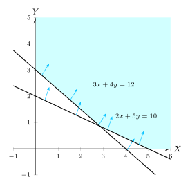
fig 7.22 — feasible region of 3x + 4y ≥ 12, 2x + 5y ≥ 10, x,y ≥ 0 …
Drawn by us to help you understand the concept clearly, and verified to make sure it's accurate. For exams, practice from your textbook's own diagram.
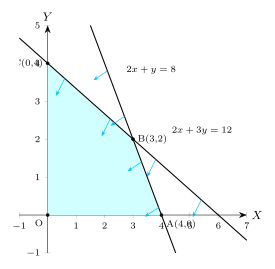
fig 7.23 — feasible region OABCO of the manufacturer problem 2x + 3y ≤ 12, 2x + y ≤ 8, x,y ≥ 0; vertices O, A(4 …