Riemann Integral

Setting up the Riemann sum. Let $f(x)$ be a real-valued, bounded function on the closed interval $[a,b]$, $a<b$. Unlike in a first geometric picture, $f(x)$ need not keep the same sign throughout $[a,b]$ — it may take both positive and negative values.

Partition $[a,b]$ into $n$ subintervals $[x_0,x_1],[x_1,x_2],\ldots,[x_{n-1},x_n]$ with

In each subinterval $[x_{i-1},x_i]$, $i=1,\ldots,n$, choose an arbitrary point $\xi_i$ with $x_{i-1}\le\xi_i\le x_i$, and form the sum

This is called a Riemann sum of $f(x)$ for the given partition. Because $\xi_i$ can be any point of $[x_{i-1},x_i]$, there are infinitely many different Riemann sums for the same partition.

Definition of the Riemann (definite) integral. If, as $n\to\infty$ with $\max(x_i-x_{i-1})\to0$ (the widest subinterval shrinking to zero), the sum in (1) tends to a single finite value $A$ — regardless of how the partition and the points $\xi_i$ were chosen — then $A$ is called the definite integral of $f$ with respect to $x$ on $[a,b]$, also called the Riemann integral, denoted

read "the integral of $f(x)$ with respect to $x$ from $a$ to $b$". When $a=b$, $\displaystyle\int_a^a f(x)\,dx=0$.

Three standard choices of the evaluation point $\xi_i$ (all yield the same limit for continuous $f$, but give different finite-$n$ approximations):

• Left-end rule ($\xi_i=x_{i-1}$): $\displaystyle\int_a^b f(x)\,dx=\lim_{n\to\infty}\sum_{i=1}^n f(x_{i-1})(x_i-x_{i-1})$.
• Right-end rule ($\xi_i=x_i$): $\displaystyle\int_a^b f(x)\,dx=\lim_{n\to\infty}\sum_{i=1}^n f(x_i)(x_i-x_{i-1})$.
• Mid-point rule ($\xi_i=\tfrac12(x_{i-1}+x_i)$): $\displaystyle\int_a^b f(x)\,dx=\lim_{n\to\infty}\sum_{i=1}^n f\!\left(\tfrac{x_{i-1}+x_i}2\right)(x_i-x_{i-1})$.

Exercise 9.1 uses each rule without taking the limit — i.e. computes just one finite Riemann sum $S=\sum f(\xi_i)\Delta x$ from a given 5-point partition of $[1,1.5]$ — which is only an approximate value of the true integral (worked in the text as Example 9.1, estimating $\int_0^{0.5}x^2\,dx$ via all three rules on 5 equal subintervals of width $h=0.1$).

Remarks connecting sign and area (used throughout §9.8):

1. If $\int_a^b f(x)\,dx$ exists, then $F(x)=\int_a^x f(u)\,du$ is a well-defined function on $[a,b]$.
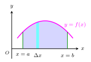
2. If $f(x)\ge0$ throughout $[a,b]$, $\int_a^b f(x)\,dx$ equals the geometric area between $y=f(x)$, the $x$-axis, and $x=a,\,x=b$.
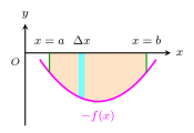
3. If $f(x)\le0$ throughout $[a,b]$, $\int_a^b f(x)\,dx$ equals the negative of that geometric area — the area itself is $-\int_a^b f(x)\,dx$. …