Hypothesis

To make a decision about a population, we first need something concrete to test — an assumption, which may turn out true or false, called a hypothesis. A hypothesis is simply a tentative, declarative statement about how two or more variables relate. Every hypothesis test works with a pair of competing statements that take opposite positions.

The null hypothesis ($H_0$) claims there is no difference — between a parameter and some specific value, or between two parameters — asserting, in effect, that the groups being compared are the same. The alternative hypothesis ($H_1$) claims the opposite: that a real difference exists, and the groups being compared are not the same.

These are written using standard comparison symbols. $H_0$ typically states equality ($=$), or a "greater than or equal to" / "less than or equal to" bound ($\geq$ or $\leq$); $H_1$ takes the complementary claim — not equal ($\neq$), strictly less than ($<$), or strictly greater than ($>$) — depending on which bound $H_0$ used. A hypothesis test never proves $H_0$ true; it only ever gives grounds to reject it in favour of $H_1$, or to fail to reject it.

Writing a null hypothesis

When two methods or treatments are being compared, any directional claim — that one is better, or worse, than the other — carries a built-in preference and so tends to be biased. The safest starting point is therefore the neutral position of no difference. If cakes baked by a conventional method have an average life of $\mu_0$ days and a new baking process is to be tested, the null hypothesis is simply $H_0: \mu = \mu_0$. Likewise, a store that will launch its own shopping app only if more than 60% of its customers shop online sets $H_0:$ (proportion using the internet $\leq 60\%$) against $H_1:$ (proportion $> 60\%$); if $H_0$ is rejected, the app is introduced.

Activity. Identify the type of each claim below and write its hypotheses $(H_0, H_1)$ in terms of the appropriate parameter ($\mu$ or $p$):

• (i) During the COVID-19 pandemic, the chance of a school student getting infected is under $25\%$.
• (ii) Fewer than $7\%$ of students ride a two-wheeler to reach school on time.
• (iii) The average salary package for Delhi University graduates is at least ₹10,00,000/annum.

Standard Error of the Mean (SEM)

Any one sample is only one of many that could have been drawn, and different samples give different means. The standard error of the mean measures how much those sample means are likely to scatter about the true population mean — in effect, it is the standard deviation of the sampling distribution of the mean:

A small SEM arises from a large number of observations that lie close to the sample mean (large $N$, small SD), which gives us confidence that the sample mean estimates the population mean relatively accurately. A large SEM arises from few, widely-varying observations (small $N$, large SD), so the estimate of the population mean is likely to be inaccurate.

Degrees of freedom

The degrees of freedom is the number of independent pieces of information on which an estimate is based — equivalently, the number of values that are free to vary once the estimate has been fixed. For example, in a class of $30$ seats the first $29$ students may choose freely but the last seat is forced, so there are $29$ degrees of freedom; scheduling three one-hour tasks in three one-hour slots leaves only two free choices, giving $2$ degrees of freedom. For a sample of size $N$,

A higher degree of freedom generally reflects a larger sample and means more power to reject a false null hypothesis and detect a genuine effect.

The t-test and the t-ratio

The t-test is a statistical test for the mean of a population, used when the population is normally (or approximately normally) distributed and its variance is unknown. The statistic it computes is the t-ratio, denoted $t$: the larger $|t|$ is, the more likely we are to reject the null hypothesis, because a large $|t|$ is stronger evidence that the groups genuinely differ. The $t$ statistic is precisely what decides whether $H_0$ should be rejected.

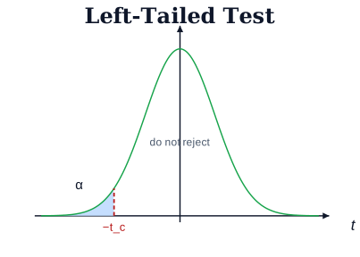
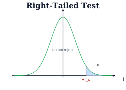
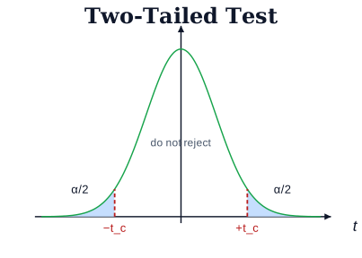
Use a two-tailed test when you only need to know whether two populations differ; use a one-tailed test when you need to know specifically whether one mean is greater than (or less than) the other. The traditional testing procedure has five steps:

1. State the hypotheses ($H_0$ and $H_1$).
2. Find the critical value(s) from the t-table.
3. Compute the test value (the t-ratio).
4. Make the decision to reject or not reject the null hypothesis.
5. Summarize the results.

Reading the t-table …