Applied Mathematics · Ch 7 — Inferential Statistics
T- Test for Two Independent Groups
T- Test for Two Independent Groups
The two-sample (independent-groups) t-test extends the same logic to comparing two groups against each other — an experimental group against a control group, say — to check whether their means differ by more than random chance would explain. A typical hypothesis pair looks like:
(the two population means are equal)
(the two population means are not equal)
The exact test statistic depends on whether the two populations are assumed to share the same variance.
Case 1 — variances assumed equal. The two samples are pooled into a single combined estimate of variability, , before computing :
where and are the two sample standard deviations, and (the pooled standard deviation) blends them into one combined estimate.
Case 2 — variances assumed unequal. No pooling is done; each sample's own variance is used directly:
Degrees of freedom also work differently in the two cases. Under equal variances, . Under unequal variances, is computed from a more elaborate expression combining both sample variances and sizes, and is generally rounded down to a whole number.
As with the one-sample test, the calculated is compared against the critical value from the t-distribution table at the chosen confidence level and degrees of freedom — if the calculated value exceeds the critical value, the null hypothesis of equal means is rejected.
Critical t-Values (t-Distribution Table)
The table below lists the critical values of the -distribution, transcribed from the t-table printed in the chapter. The top row is the area in one tail (the significance level for a one-tailed test); the italic row beneath it is the matching area in two tails (use it for a two-tailed test). Each row is a value of the degrees of freedom . To find a critical , read down to your and across to the appropriate column; for a left-tailed test the value is negative, for a right-tailed test positive, and for a two-tailed test both signs () apply. For example, at the two-tailed critical value is , and the one-tailed value is .
| / one-tail | 0.005 | 0.01 | 0.025 | 0.05 | 0.10 |
|---|---|---|---|---|---|
| (two-tail ) | 0.01 | 0.02 | 0.05 | 0.10 | 0.20 |
| 1 | 63.657 | 31.821 | 12.706 | 6.314 | 3.078 |
| 2 | 9.925 | 6.965 | 4.303 | 2.920 | 1.886 |
| 3 | 5.841 | 4.541 | 3.182 | 2.353 | 1.638 |
| 4 | 4.604 | 3.747 | 2.776 | 2.132 | 1.533 |
| 5 | 4.032 | 3.365 | 2.571 | 2.015 | 1.476 |
| 6 | 3.707 | 3.143 | 2.447 | 1.943 | 1.440 |
| 7 | 3.499 | 2.998 | 2.365 | 1.895 | 1.415 |
| 8 | 3.355 | 2.896 | 2.306 | 1.860 | 1.397 |
| 9 | 3.250 | 2.821 | 2.262 | 1.833 | 1.383 |
| 10 | 3.169 | 2.764 | 2.228 | 1.812 | 1.372 |
| 11 | 3.106 | 2.718 | 2.201 | 1.796 | 1.363 |
| 12 | 3.055 | 2.681 | 2.179 | 1.782 | 1.356 |
| 13 | 3.012 | 2.650 | 2.160 | 1.771 | 1.350 |
| 14 | 2.977 | 2.624 | 2.145 | 1.761 | 1.345 |
| 15 | 2.947 | 2.602 | 2.131 | 1.753 | 1.341 |
| 16 | 2.921 | 2.583 | 2.120 | 1.746 | 1.337 |
| 17 | 2.898 | 2.567 | 2.110 | 1.740 | 1.333 |
| 18 | 2.878 | 2.552 | 2.101 | 1.734 | 1.330 |
| 19 | 2.861 | 2.539 | 2.093 | 1.729 | 1.328 |
| 20 | 2.845 | 2.528 | 2.086 | 1.725 | 1.325 |
| 21 | 2.831 | 2.518 | 2.080 | 1.721 | 1.323 |
| 22 | 2.819 | 2.508 | 2.074 | 1.717 | 1.321 |
| 23 | 2.807 | 2.500 | 2.069 | 1.714 | 1.319 |
| 24 | 2.797 | 2.492 | 2.064 | 1.711 | 1.318 |
| 25 | 2.787 | 2.485 | 2.060 | 1.708 | 1.316 |
| 26 | 2.779 | 2.479 | 2.056 | 1.706 | 1.315 |
| 27 | 2.771 | 2.473 | 2.052 | 1.703 | 1.314 |
| 28 | 2.763 | 2.467 | 2.048 | 1.701 | 1.313 |
| 29 | 2.756 | 2.462 | 2.045 | 1.699 | 1.311 |
| 30 | 2.750 | 2.457 | 2.042 | 1.697 | 1.310 |
| 31 | 2.744 | 2.453 | 2.040 | 1.696 | 1.309 |
| 32 | 2.738 | 2.449 | 2.037 | 1.694 | 1.309 |
| 34 | 2.728 | 2.441 | 2.032 | 1.691 | 1.307 |
| 36 | 2.719 | 2.434 | 2.028 | 1.688 | 1.306 |
| 38 | 2.712 | 2.429 | 2.024 | 1.686 | 1.304 |
| 40 | 2.704 | 2.423 | 2.021 | 1.684 | 1.303 |
| 45 | 2.690 | 2.412 | 2.014 | 1.679 | 1.301 |
| 50 | 2.678 | 2.403 | 2.009 | 1.676 | 1.299 |
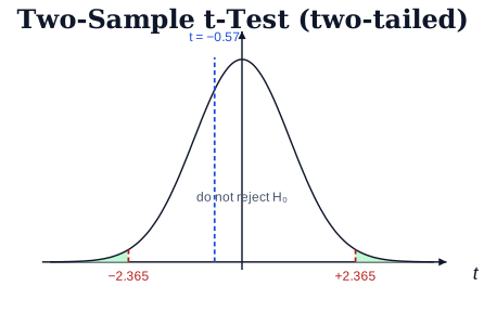
Drawn by us to help you understand the concept clearly, and verified to make sure it's accurate. For exams, practice from your NCERT textbook's own diagram.
The obtained t = −0.57 lies inside ±2.365, in the do-not-reject region, so H₀ i …