Physics · Ch 3 — Current Electricity

Drift of Electrons and the Origin of Resistivity

3.5

Drift of Electrons and the Origin of Resistivity

Why Electrons Drift (and Don't Just Accelerate Forever)

In a metal, free electrons are in constant, random motion, colliding with the fixed positive ions. Without an electric field, these collisions randomise velocities so thoroughly that the average velocity of all electrons is zero:

\frac{1}{N} \sum_{i=1}^{N} \mathbf{v}_i = 0

When an electric field $\mathbf{E}$ is applied, each electron experiences a constant acceleration:

\mathbf{a} = -\frac{e}{m} \mathbf{E}

where $e$ is the magnitude of the electron charge and $m$ is its mass. The negative sign indicates the acceleration is opposite to the field direction.

The Key Idea: Relaxation Time

Between collisions, an electron accelerates. Immediately after a collision, its velocity is random. If the $i$ -th electron had its last collision a time $t_i$ ago, its velocity at the present instant is:

\mathbf{V}_i = \mathbf{v}_i - \frac{e}{m} \mathbf{E} \, t_i

The average of $\mathbf{V}_i$ over all electrons is the drift velocity $\mathbf{v}_d$ . The average of the random $\mathbf{v}_i$ is zero. The average of the times $t_i$ is the relaxation time $\tau$ — the average time between successive collisions. This gives:

\mathbf{v}_d = \langle \mathbf{V}_i \rangle = 0 - \frac{e}{m} \mathbf{E} \, \tau = -\frac{e \tau}{m} \mathbf{E}

The magnitude of the drift velocity is:

v_d = \frac{e \tau}{m} E

Crucial insight: Electrons do not accelerate indefinitely. Each collision resets their directed motion, so they acquire a steady, small average drift speed proportional to the field.

From Drift to Current Density

Consider a cross-sectional area $A$ perpendicular to $\mathbf{E}$ . In time $\Delta t$ , all electrons within a distance $v_d \Delta t$ to the left of $A$ will cross it. If $n$ is the number of free electrons per unit volume, the number crossing is $n (v_d \Delta t) A$ . Each carries charge $-e$ , so the total charge crossing is $-n e v_d A \Delta t$ . The magnitude of current $I$ is:

I \Delta t = n e v_d A \Delta t \quad \Rightarrow \quad I = n e v_d A

Substituting $v_d = \frac{e \tau}{m} E$ :

I = n e \left( \frac{e \tau}{m} E \right) A = \frac{n e^2 \tau}{m} E A

Since current density $j = I/A$ and $\mathbf{j}$ is parallel to $\mathbf{E}$ , we get Ohm's law in vector form:

\mathbf{j} = \frac{n e^2 \tau}{m} \mathbf{E}

Comparing with $\mathbf{j} = \sigma \mathbf{E}$ gives the microscopic expression for conductivity:

\sigma = \frac{n e^2 \tau}{m}

This derivation assumes $\tau$ and $n$ are constants (independent of $\mathbf{E}$ ), which is the basis of Ohm's law.

Important Physical Insights

Drift speed is tiny — typically $\sim 1$ mm/s for common currents, compared to thermal speeds $\sim 10^2$ m/s and field propagation speed $\sim 3 \times 10^8$ m/s.
Current establishes almost instantly because the electric field propagates at light speed, causing local drift everywhere simultaneously — electrons don't need to travel from one end to the other. …

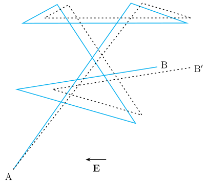
Figure 3.3A schematic picture of an electron moving from a point A to another point B through repeated collisions, and straight line travel between collisions (full lines). If an electric field is applied as shown, the electron ends up at point B′ (dotted lines). A slight drift in a direction opposite the electric field is visible.

Fig. 3.3 — A schematic picture of an electron moving from a point A to another point B through repeated collisions, and straight line travel between collisions (full lines). If an electric field is applied as shown, the electron ends up at point B′ (dotted lines). A slight drift in a direction opposite the electric field is visible.

Drawn by us to help you understand the concept clearly, and verified to make sure it's accurate. For exams, practice from your textbook's own diagram.

What the figure shows

The figure is a schematic of a single electron’s trajectory inside a metal. The solid jagged path starts at point A (lower left) and ends at point B (right). Each straight solid segment represents the electron’s motion between two successive collisions with the fixed positive ions. The sharp corners are the collision points, where the electron’s direction changes randomly. The dotted path is an overlay: it follows the same zig‑zag shape but is shifted slightly to the right, ending at point B′ (just to the right of B). A short bold horizontal arrow labelled E points to the left, indicating the direction of the applied electric field. The net displacement from A to B′ is to the right — opposite to the field direction. This illustrates the drift of the electron.

Physical idea

In the absence of an electric field, the electron’s random collisions cause its average velocity to be zero — it wanders but goes nowhere on average. When a field $\vec{E}$ is applied, the electron experiences a constant acceleration $\vec{a} = -\frac{e}{m}\vec{E}$ (since the electron’s charge is $-e$ ). Between collisions, the electron’s path curves slightly in the direction opposite to $\vec{E}$ (because the force is $-\!e\vec{E}$ ). Over many collisions, this small extra displacement per segment accumulates, producing a net drift in the direction opposite to $\vec{E}$ . The dotted path shows this net shift: the electron ends at B′ instead of B. The drift is tiny compared to the random thermal motion, but it is steady and gives rise to a current.

Key formula developed from this figure

The textbook uses the figure to derive the drift velocity:

\vec{v}_d = -\frac{e \tau}{m} \vec{E}

where:

$\vec{v}_d$ = average drift velocity of electrons (direction opposite to $\vec{E}$ )
$e$ = magnitude of electron charge ( $1.6 \times 10^{-19}$ C)
$\tau$ = average time between successive collisions (relaxation time)
$m$ = mass of an electron ( $9.1 \times 10^{-31}$ kg)
$\vec{E}$ = applied electric field

From this, the current density $\vec{j}$ is obtained: …

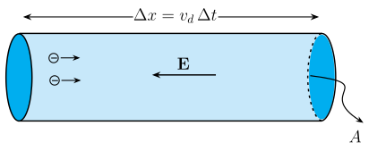
Figure 3.4Current in a metallic conductor. The magnitude of current density in a metal is the magnitude of charge contained in a cylinder of unit area and length v_d.

Fig. 3.4 — Current in a metallic conductor. The magnitude of current density in a metal is the magnitude of charge contained in a cylinder of unit area and length v_d.

Drawn by us to help you understand the concept clearly, and verified to make sure it's accurate. For exams, practice from your textbook's own diagram.

What the Figure Shows

The figure is a 3‑D schematic of a short cylindrical segment inside a metallic conductor. The cylinder is drawn as a light tube with elliptical end‑caps. At the left end, two small circles each carry a ‘–’ sign, representing electrons, and each has a tiny arrow pointing right — this indicates the direction of electron drift. Inside the cylinder, near its centre, a bold arrow labelled E points left, showing the direction of the applied electric field. Above the cylinder, spanning its full length, a double‑headed dimension arrow is labelled Δx = v_d Δt. The right end‑face of the cylinder is labelled A with a lead‑line.

The Physical Idea

The figure illustrates how a steady current arises from the drift of electrons. Even though individual electrons move randomly, an applied electric field E (pointing left) causes them to acquire a small average velocity v_d (drift velocity) in the opposite direction (right). In a time interval Δt, all electrons that lie within a distance v_d Δt to the left of area A will cross that area. The cylinder of length v_d Δt and cross‑sectional area A therefore contains the charge that flows through A in time Δt.

Key Formula Derived from This Figure

The total charge crossing area A in time Δt is the charge contained in the cylinder:

\Delta Q = -e \times (n \times \text{volume}) = -e \, n \, (A \, v_d \, \Delta t)

where:

$e$ = magnitude of electron charge ( $1.6 \times 10^{-19}$ C)
$n$ = number of free electrons per unit volume (m $^{-3}$ )
$A$ = cross‑sectional area (m $^2$ )
$v_d$ = drift speed (m/s)
$\Delta t$ = time interval (s)

Since current $I = \Delta Q / \Delta t$ (magnitude), we get the drift‑current relation:

$I = n e A v_d$ …

Start your 14-day free trial to unlock the full solution →

← Previous · 3.4Ohm's Law Next · 3.5 →Example 3.1 — (a) Estimate the average drift speed of conduction electrons in a copp…