Temperature Dependence of Resistivity

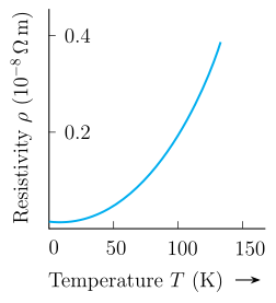
The graph plots resistivity $\rho_T$ (in units of $10^{-8} \, \Omega \, \text{m}$) on the vertical axis against absolute temperature $T$ (in kelvin) on the horizontal axis. The vertical axis is marked at $0.2$ and $0.4$ (i.e., $0.2 \times 10^{-8} \, \Omega \, \text{m}$ and $0.4 \times 10^{-8} \, \Omega \, \text{m}$). The horizontal axis has ticks at $0$, $50$, $100$, and $150$ K.

The curve begins near the origin at very low temperatures and rises with an upward-concave (parabola-like) shape. By $T \approx 150$ K, the resistivity climbs steeply toward $\rho \approx 0.4 \times 10^{-8} \, \Omega \, \text{m}$. This shows that resistivity increases with temperature for copper, but the increase is not linear over the entire range — especially at very low temperatures, the graph deviates from a straight line.

Physical idea: Over a limited range of temperatures (not too large), the resistivity of a metallic conductor follows the approximate linear relation:

where:

• $\rho_T$ = resistivity at temperature $T$,
• $\rho_0$ = resistivity at a reference temperature $T_0$,
• $\alpha$ = temperature coefficient of resistivity (units: $^\circ\text{C}^{-1}$ or $\text{K}^{-1}$).

For metals, $\alpha$ is positive, meaning resistivity rises with temperature. However, at temperatures much lower than $0^\circ\text{C}$ (i.e., below about 273 K), the graph deviates considerably from a straight line — as Fig. 3.8 shows with its curved shape near the origin. The linear formula is therefore only an approximation valid over a limited range around any chosen $T_0$. …

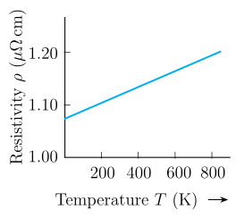
The graph plots resistivity $\rho_T$ (in units of $\mu\Omega\,\text{cm}$) on the vertical axis against absolute temperature $T$ (in kelvin) on the horizontal axis. The vertical scale runs from $1.00$ to $1.20\ \mu\Omega\,\text{cm}$, and the horizontal scale from $200$ to $800\ \text{K}$.

The data form a nearly straight line with a gentle positive slope. At low temperatures (near $200\ \text{K}$) the resistivity is about $1.08\ \mu\Omega\,\text{cm}$, rising to about $1.20\ \mu\Omega\,\text{cm}$ at $800\ \text{K}$. This weak, almost-linear increase contrasts sharply with the curved plot for copper shown in the textbook’s Fig. 3.8.

Physical idea: Nichrome is an alloy (nickel, iron, chromium) whose resistivity changes very little with temperature. This makes it ideal for wire-wound standard resistors and heating elements, because its resistance remains nearly constant over a wide temperature range.

Key formula developed with this figure is the linear approximation for resistivity over a limited temperature range:

• $\rho_T$ = resistivity at temperature $T$
• $\rho_0$ = resistivity at reference temperature $T_0$
• $\alpha$ = temperature coefficient of resistivity (units: $^\circ\text{C}^{-1}$ or $\text{K}^{-1}$) …

What the Graph Shows

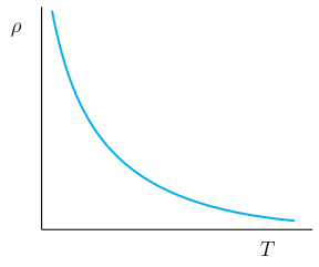
The figure is a first-quadrant plot with resistivity $\rho$ on the vertical axis and temperature $T$ on the horizontal axis. There are no numeric ticks — it is a schematic (conceptual) graph.

The curve begins at a high value of $\rho$ when $T$ is small (near the vertical axis). As $T$ increases, the curve falls steeply, then gradually flattens out and approaches the $T$-axis asymptotically. The shape is that of an exponential decay: resistivity decreases rapidly at first, then more slowly, and eventually tends toward a very low, nearly constant value.

The Physical Idea

This graph illustrates the opposite behaviour of semiconductors compared to metals. For metals, resistivity increases with temperature (positive temperature coefficient). For semiconductors, resistivity decreases with temperature (negative temperature coefficient).

The reason lies in the number of charge carriers $n$. In a semiconductor, raising the temperature dramatically increases $n$ — more electrons break free from their bonds and become available for conduction. This increase in $n$ more than compensates for the decrease in the average collision time $\tau$ (which also occurs because electrons move faster). The net effect is that $\rho$ drops sharply.

The Key Formula

The textbook derives resistivity from the relation:

where:

• $m$ = mass of an electron
• $n$ = number of free electrons per unit volume …