Electronics · Ch 6 — Oscillators
Introduction
Introduction
An oscillator is an electronic circuit that converts DC energy into AC energy of a desired frequency. The AC sources it produces range from a few hertz to several gigahertz, which is why oscillators sit at the heart of radios, TV transmitters and receivers, radar sets, computers and many other electronic devices.
Classification of oscillators
Oscillators are grouped in two ways:
- By the shape of the waveform they generate — (i) sinusoidal oscillators and (ii) non-sinusoidal oscillators.
- By the components used in the feedback circuit — sinusoidal oscillators are further divided into (i) LC oscillators, (ii) RC oscillators and (iii) crystal oscillators.
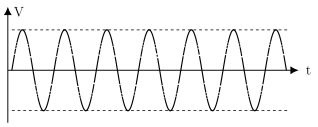
Sinusoidal (harmonic) oscillator. When the output is a smooth sine wave of constant amplitude the circuit is a sinusoidal, or harmonic, oscillator (Figure 6.1.1).
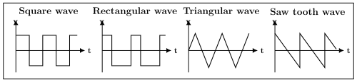
Non-sinusoidal oscillator. When the output is some other repeating shape — square, rectangular, triangular or saw-tooth — the circuit is a non-sinusoidal oscillator (Figure 6.1.2).
Damped and un-damped oscillations
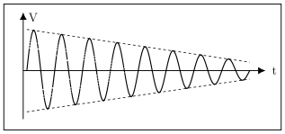
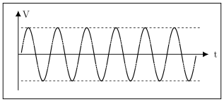
Damped oscillations are electrical oscillations whose amplitude keeps decreasing with time while the frequency stays the same (Figure 6.1.3). Un-damped (sustained) oscillations are oscillations whose amplitude stays constant with time — both amplitude and frequency remain unchanged (Figure 6.1.4). A useful oscillator must deliver sustained oscillations, so the whole design problem is to keep the amplitude from decaying.
Basic principle of an oscillator
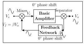
An oscillator is an amplifier with positive feedback. Feedback is positive when the feedback voltage returned to the input is in phase with the input signal. Consider the amplifier-plus-feedback arrangement of Figure 6.1.5, where the loop is drawn with 0 degrees phase shift in both the forward and feedback paths.
The open-loop gain of the amplifier is . After positive feedback the overall gain is . Because the amplifier input is the sum of the source and feedback voltages, , and the feedback voltage is , we get . Substituting and dividing numerator and denominator by gives the closed-loop gain
Here is called the loop gain and is the feedback ratio.
Stabilization of oscillations
The expression contains the necessary condition for sustained oscillations. If the loop gain reaches , the denominator becomes zero and : the circuit produces an output with no input applied. In other words, the amplifier has become an oscillator.
Start-up oscillations and start-up conditions
Where does the very first signal come from if there is no input? The starting voltage is provided by noise — the random thermal movement of free electrons in the circuit resistors at room temperature. When power is switched on, this tiny noise voltage is amplified, drives the feedback network, and returns to the input. If the feedback network is designed so that the total loop phase shift is 0 degrees (equivalently 360 degrees), the signal reinforces itself at one frequency and grows into a steady oscillation.
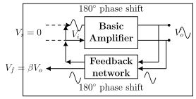
In a typical transistor oscillator the inverting amplifier contributes 180 degrees and the feedback network contributes another 180 degrees, giving 360 degrees around the loop (Figure 6.1.6). At switch-on the loop gain is deliberately greater than 1, so the oscillations build up; as the amplitude rises the amplifier gain falls until settles at exactly 1, giving a constant-amplitude output.
Treating a fictitious input applied to the amplifier: the output is and the feedback voltage . For a true oscillator the external source is removed (), so the feedback voltage alone sustains the input, , which requires with in phase with .
Barkhausen criterion
The two conditions above are summarised as the Barkhausen criterion for sustained oscillations:
- The total phase shift around the closed loop must be 0 degrees (or 360 degrees).
- The magnitude of the loop gain must be unity, .
The value of the loop gain decides the nature of the oscillations: …
An oscillator is an electronic circuit that converts DC energy into AC energy of a desired frequency, producing an AC output (a few Hz up to several GHz) with no externally applied AC input. It is an amplifier with positive feedback that draws energy from a DC supply and delivers a continuous AC waveform, which is why oscillators …
A sinusoidal or harmonic oscillator produces an output that is a continuous sine wave of constant amplitude and single frequency. Its waveform is a smooth, un-damped sine wave, and by the components used in the feedback network these harmonic oscillators are …
Drawn by us to help you understand the concept clearly, and verified to make sure it's accurate. For exams, practice from your textbook's own diagram.
Figure 6.1.1 shows the output of a sinusoidal oscillator: a smooth sine wave of constant amplitude on V (vertical) versus t (horizontal) axes, with dashed horizontal envelope lines marking the equal positive and negative peaks. It illustrates what a h …
A non-sinusoidal oscillator produces a repeating output of a shape other than a sine wave — for example square, rectangular, triangular or saw-tooth. Such repeating waveforms come from relaxation-type circuits rather than a tuned tank circuit; in this chapter the 555 timer is the standar …
Drawn by us to help you understand the concept clearly, and verified to make sure it's accurate. For exams, practice from your textbook's own diagram.
Figure 6.1.2 shows the four non-sinusoidal output shapes side by side, each on its own v-vs-t axes: a square wave, a rectangular pulse train (unequal high/low times), a triangular wave and a saw-tooth wave. It contrasts the outputs of non-sinusoidal oscillat …
Electrical oscillations whose amplitude keeps decreasing with time while the frequency of oscillation stays the same are called damped oscillations. They occur when the loop gain is below unity, , or when resistive, radiation and dielectric losses drain energy each cycle, so a practical osci …
Drawn by us to help you understand the concept clearly, and verified to make sure it's accurate. For exams, practice from your textbook's own diagram.
Figure 6.1.3 shows damped oscillations: a sine wave on V-vs-t axes whose amplitude falls progressively from left to right, with two dashed straight envelope lines converging toward the time axis (decaying amplitude, constant frequency). The same waveform is repeate …
Electrical oscillations whose amplitude remains constant with time are called un-damped or sustained oscillations; both the amplitude and the frequency stay constant. A practical oscillator mu …
Drawn by us to help you understand the concept clearly, and verified to make sure it's accurate. For exams, practice from your textbook's own diagram.
Figure 6.1.4 shows un-damped (sustained) oscillations: a sine wave on V-vs-t axes of constant amplitude, with dashed horizontal envelope lines at fixed positive and negative peaks. The same waveform is repeated later …
Feedback is positive when the feedback voltage returned to the amplifier input is in phase with the input signal. Positive feedback is the essential condition that turns a …
Drawn by us to help you understand the concept clearly, and verified to make sure it's accurate. For exams, practice from your textbook's own diagram.
Figure 6.1.5 is the block diagram used to derive the feedback gain: source voltage Vs enters a mixer, the mixer output Vi drives the basic amplifier to give Vo through a separator, and a feedback network of ratio beta returns Vf = beta*Vo to the mixer, with 0 degrees phase shift marked on both the forward and feedback …
, where is the open-loop gain, the feedback ratio and the loop gain. When the gain : the amplifier delivers an output wi …
Drawn by us to help you understand the concept clearly, and verified to make sure it's accurate. For exams, practice from your textbook's own diagram.
Figure 6.1.6 shows the oscillator block diagram with the external source removed (Vs = 0): the basic amplifier contributes 180 degrees and the feedback network another 180 degrees, so the loop phase shift totals 360 degrees, and the feedback voltage Vf = beta*Vo alone sustains the inpu …
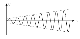
For sustained oscillations: (1) the total phase shift around the closed loop is 0 degrees or 360 degrees, and (2) the magnitude of the loop gain is unity, . If the oscillations are damped, if they gro …
Drawn by us to help you understand the concept clearly, and verified to make sure it's accurate. For exams, practice from your textbook's own diagram.
Figure 6.1.7 shows the case A*beta < 1: a sine wave whose amplitude decays with time (converging dashed envelope) inside a rectangular border. It is the same damped waveform as Figure 6.1.3, shown here to illustrate …
Drawn by us to help you understand the concept clearly, and verified to make sure it's accurate. For exams, practice from your textbook's own diagram.
Figure 6.1.8 shows the case A*beta > 1: a sine wave whose amplitude increases progressively with time, with two dashed envelope lines diverging away from the time axis, inside a rectangular border. It correctly depicts growing (building-up) oscillations, despite the caption text …
Drawn by us to help you understand the concept clearly, and verified to make sure it's accurate. For exams, practice from your textbook's own diagram.
Figure 6.1.9 shows the case A*beta = 1: a sine wave of constant amplitude (parallel dashed envelope lines) inside a rectangular border. It is the same sustained waveform as Figure 6.1.4, illustrating the loop-ga …