Mathematics · Ch 7 — Linear Programming
Solution of L.P.P. by graphical methods
Solution of L.P.P. by graphical methods
Formal definitions related to L.P.P.:
-
Solution of an L.P.P. — a set of values of the decision variables which satisfies the
conditions of the given L.P.P. is called a solution to that problem.
-
Feasible solution — a solution which satisfies ALL the given constraints (including non-negativity) is called a
feasible solution.
-
Optimal feasible solution — a feasible solution which maximizes or minimizes the objective function, as required
by the problem, is called an optimal feasible solution.
-
Feasible region — the region of the plane determined by (common to) ALL the constraints of the L.P.P. is called
the feasible region.
There are two standard methods to find the solution of an L.P.P.: the Graphical method and the Simplex method;
this chapter restricts itself entirely to the graphical method, which only works conveniently for at most two decision
variables.
Two theorems (stated without proof), the foundation of the graphical method:
- Theorem 1: the set of all feasible solutions of an L.P.P. — the feasible region — is a convex set.
- Theorem 2 (Convex Polygon Theorem): the objective function of an L.P.P. attains its optimum value (maximum or minimum) at (at least) one of the vertices of the convex polygon that is the feasible region.
The Corner-Point Method — five steps:
- Convert every inequation constraint into its boundary equation.
- Draw each boundary line in the – plane.
- Locate the region common to all the constraints — this is the feasible region.
- Find every vertex (corner point) of the feasible region.
- Evaluate the objective function at every vertex found; the largest value is the maximum and the smallest is the minimum of over the whole feasible region.
The reasoning behind step 5 is that the feasible region, being a convex region bounded by straight lines, can be swept by
imagining the line (an "iso-value" line of the objective ) sliding across the plane as varies —
the LAST point of the feasible region this sweeping line touches (for a maximum) or the FIRST point it touches (for a
minimum) is always a vertex of the polygon, unless the sweeping line becomes exactly parallel to one whole edge, in which
case every point of that edge is simultaneously optimal.
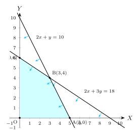
Solved Example 1 — an ordinary bounded maximum. Maximize subject to . Draw (through and ) and (through and ); testing the
origin, both constraints shade their origin side. The feasible region has vertices , (on ),
(solving and together: from , ; substituting into , ), and (on ). Evaluating : , ,
, . The maximum value is , occurring at , i.e. .
Drawn by us to help you understand the concept clearly, and verified to make sure it's accurate. For exams, practice from your textbook's own diagram.
fig 7.24 — feasible region OABC for maximizing z = 9x + 13y; vertices O, A(5,0), …
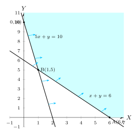
Solved Example 2 — a mislabelled optimization (the textbook's own worked example, reproduced honestly). The text
states: "Maximize subject to ." Its feasible region has vertices
, , , tabulated as . Since BOTH constraints only impose LOWER
() bounds with no matching upper cap, this region is actually unbounded toward increasing and — for
example, still satisfies and , giving , far larger than any of the three
tabulated vertex values. So if is genuinely to be MAXIMIZED here, no finite maximum exists at all. What the text's own
working actually computes is the SMALLEST of the three tabulated values, at — which is exactly what a
MINIMIZATION of the same objective over the same region would give (minimizing over a region that is bounded below, even
though unbounded above, does have a genuine finite optimum at a vertex). This strongly suggests the problem was intended
to read "Minimize," and the printed "maximum value of " is very likely a proofreading slip for "minimum value" —
this platform reports both readings rather than silently reproducing a number that does not actually answer the stated
problem: as literally printed (Maximize), the true answer is "unbounded, no finite maximum"; as very likely intended
(Minimize), the answer is at , matching the book's own corner-point table.
Drawn by us to help you understand the concept clearly, and verified to make sure it's accurate. For exams, practice from your textbook's own diagram.
fig 7.25 — unbounded feasible region for z = 5x + 2y (5x + y ≥ 10, x + y ≥ 6); corner points A(6,0) …
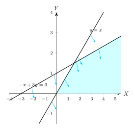
Solved Example 3 — the unbounded, no-finite-maximum case. Maximize subject to . Drawing and (through and ), the common shaded region is
unbounded (not a closed polygon) — it opens up indefinitely toward increasing (and correspondingly increasing ,
staying above the line ). In such a case the iso-value line can be slid further and further from the
origin, always finding more of the feasible region to cross, so can be made as large as desired: there is NO finite
maximum value of within this feasible region. This is the chapter's own explicit demonstration that boundedness of
the feasible region (section 7.1.1's convex-set note (ii), revisited) is not just a technical curiosity but something
that must be checked before declaring any "maximum" answer.
Drawn by us to help you understand the concept clearly, and verified to make sure it's accurate. For exams, practice from your textbook's own diagram.
fig 7.26 — unbounded feasible region for z = 3x + 4y (x − y ≥ 0, −x + 3y ≤ 3): no …
…
| Vertex of | Value of at |
|---|---|
| O (0, 0) | 0 |
| A (5, 0) | 45 |
| Vertex | |
|---|---|
| O (0, 0) | 0 |
| A (2, 0) | 10 |
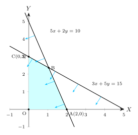
Worked out. A short explanatory remark accompanies the Corner-Point Method: since the feasible region is a convex region bounded by straight lines, if a linear objective is optimized somewhere in the region, that point must be a vertex of the polygon — this can be pictured (verified, in the book's own words) by imagining the line sweeping across the feasible region as the constant is varied, touching the region last (for a maximum) or first (for a minimum) exactly at a corner rather than along a whole edge, …
Drawn by us to help you understand the concept clearly, and verified to make sure it's accurate. For exams, practice from your textbook's own diagram.
fig 7.27 — feasible region OABC for z = 5x + 2y; vertices O, A(2,0), B(20/19, 4 …