Hysteresis

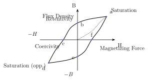
The behaviour of a ferromagnetic material subjected to a changing external field is markedly NON-LINEAR, and, unlike a simple linear material, it carries a memory of its past magnetic history -- this behaviour is called hysteresis. To study it, consider an initially unmagnetised ferromagnetic rod placed inside a solenoid, so that passing a current through the solenoid generates a magnetising field $H=nI$ that progressively magnetises the rod; knowing the material's susceptibility (where it applies) or measuring directly, the resulting magnetization M and total field B can be tracked as the current -- and hence H -- is varied through one complete cycle (Fig. 11.11).

Starting from the unmagnetised state at the origin O, as H is increased from zero, B rises but NON-linearly, following a dotted (first-magnetisation) curve, until near point a, B reaches a maximum, saturation value: essentially all the domains have merged into one, fully aligned domain (as described in section 11.5.3), and further increasing H produces no further increase in B. Crucially, this magnetisation process is NOT reversible: when the current (and hence H) is now reduced, the curve does NOT retrace its earlier path back toward the origin, because the domain structure that formed on the way up does not simply undo itself. When H is brought all the way back to zero (point b), B is found to be NOT zero -- some domain alignment persists even with no applied field at all. This leftover value of B, at $H=0$, is called the retentivity or remanence of the material.

Continuing the cycle, the current in the solenoid is now increased in the REVERSED direction. As the reversed H grows, B falls further, passing through zero at point c, where B first returns to zero at a certain (reversed) value of H -- this required reversed field strength is called the coercivity of the material. At this point, the domain axes are essentially randomly oriented again. Increasing the reversed field further, B grows in magnitude (now in the reversed sense) until it again reaches a saturation value at point d, symmetric to point a but in the opposite direction; beyond d, further increasing the reversed H produces no further change in B.

Reducing this reversed H back toward zero, B falls along a new path to point e, where once again $H=0$ but $B\neq0$ -- the same retentivity magnitude as at b, but now in the reversed sense, meaning the domain structure is present but the overall direction of magnetisation has flipped. Finally, increasing H once more in the original (positive) direction carries the curve back up through point f (where B again returns to zero, at the ORIGINAL coercivity value of H) and on to point a, completing the loop. This entire closed B-H curve is the hysteresis loop, and carrying a ferromagnetic sample through it once is called a hysteresis cycle. …