Distance between skew lines

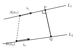
Theorem 6.6 (Distance between skew lines). If line $L_1$ has vector equation $\vec r = \vec a_1 + \lambda_1 \vec b_1$ and line $L_2$ has vector equation $\vec r = \vec a_2 + \lambda_2 \vec b_2$, then the shortest distance between $L_1$ and $L_2$ is

Proof (outline). Let $L_1$ pass through the point $A(\vec a_1)$ in the direction $\vec b_1$, and let $L_2$ pass through $B(\vec a_2)$ in the direction $\vec b_2$. Let $PQ$ be the unique line segment perpendicular to both $L_1$ and $L_2$, with $P$ on $L_1$ and $Q$ on $L_2$ (see Fig. 6.6) -- this is exactly the segment whose length is the shortest distance we want. Since $PQ$ is perpendicular to both $\vec b_1$ and $\vec b_2$, it must be parallel to $\vec b_1\times\vec b_2$, because the cross product of two vectors is, by definition, perpendicular to both of them. So the unit vector along $PQ$ is $\hat n = \dfrac{\vec b_1\times\vec b_2}{|\vec b_1\times\vec b_2|}$.

Now $PQ$ is the length of the projection of $\overrightarrow{AB}$ along $\hat n$, i.e. $PQ = \overrightarrow{AB}\cdot\hat n$. Since $\overrightarrow{AB} = \vec a_2-\vec a_1$, this gives

and taking the modulus (distance is never negative) gives the formula of Theorem 6.6.

Remark -- the intersection test. Two lines intersect each other if and only if the shortest distance between them is zero. Combined with Theorem 6.6, this means that lines $\vec r=\vec a_1+\lambda_1\vec b_1$ and $\vec r=\vec a_2+\lambda_2\vec b_2$ intersect each other if and only if

In Cartesian form, if the lines are $\dfrac{x-x_1}{a_1}=\dfrac{y-y_1}{b_1}=\dfrac{z-z_1}{c_1}$ and $\dfrac{x-x_2}{a_2}=\dfrac{y-y_2}{b_2}=\dfrac{z-z_2}{c_2}$, they intersect each other if and only if

This determinant is exactly the scalar triple product $(\vec a_2-\vec a_1)\cdot(\vec b_1\times\vec b_2)$ written out in coordinates -- the same test in a different notation, useful when the lines are given directly in symmetric (Cartesian) form instead of vector form. If a pair of lines is neither parallel nor satisfies this condition, the lines are skew.

Ex.(14) Find the shortest distance between lines $\vec r=(2\hat i-\hat j)+\lambda(2\hat i+\hat j-3\hat k)$ and $\vec r=(\hat i-\hat j+2\hat k)+\mu(2\hat i+\hat j-5\hat k)$

Solution. Here $\vec a_1=2\hat i-\hat j$, $\vec a_2=\hat i-\hat j+2\hat k$, $\vec b_1=2\hat i+\hat j-3\hat k$, $\vec b_2=2\hat i+\hat j-5\hat k$.

Ex.(15) Find the shortest distance between lines $\dfrac{x-1}{2}=\dfrac{y-2}{3}=\dfrac{z-3}{4}$ and $\dfrac{x-2}{3}=\dfrac{y-4}{4}=\dfrac{z-5}{5}$

Solution. The vector forms of the given lines are $\vec r=(\hat i+2\hat j+3\hat k)+\lambda(2\hat i+3\hat j+4\hat k)$ and $\vec r=(2\hat i+4\hat j+5\hat k)+\mu(3\hat i+4\hat j+5\hat k)$, so $\vec a_1=\hat i+2\hat j+3\hat k$, $\vec a_2=2\hat i+4\hat j+5\hat k$, $\vec b_1=2\hat i+3\hat j+4\hat k$, $\vec b_2=3\hat i+4\hat j+5\hat k$.

$\vec b_1\times\vec b_2=\begin{vmatrix}\hat i&\hat j&\hat k\\2&3&4\\3&4&5\end{vmatrix}=-\hat i+2\hat j-\hat k,\qquad |\vec b_1\times\vec b_2|=\sqrt{1+4+1}=\sqrt6$ …