Mathematics · Ch 4 — Pair of Straight Lines
Homogeneous equation of degree two
Homogeneous equation of degree two
A homogeneous equation of degree two in and has the general form . This section shows exactly when such an equation is the combined equation of a pair of lines through the origin, and how to recover the slopes of those lines.
Theorem 4.2. The combined equation of a pair of lines passing through the origin is a homogeneous equation of degree two in and .
Proof. Let and be any two lines through the origin.
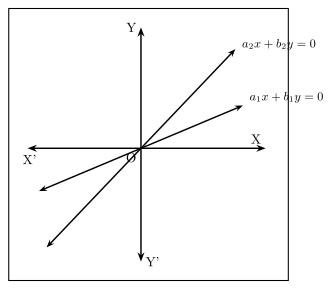
Drawn by us to help you understand the concept clearly, and verified to make sure it's accurate. For exams, practice from your textbook's own diagram.
What this figure shows. A coordinate-axis sketch (X'X horizontal, Y'Y vertical, origin O marked at the centre) showing two straight lines drawn through the origin, labelled by their separate equations and . The picture accompanies the Case-1 argument of the pair-of-lines test (the case b = 0), and simply illustrates that both lines pass through O -- it does not give away the algebraic working that follow …
Their combined equation is , which expands to . Writing , , and , this is exactly , a homogeneous equation of degree two (every term -- , , -- has degree two).
The converse is not automatic: every homogeneous equation of degree two need not represent a real pair of lines. For instance is homogeneous of degree two, but its only real solution is the single point , not two lines. The next theorem pins down exactly when a homogeneous equation does represent a genuine pair of lines.
Theorem (the test). The homogeneous equation represents a pair of lines through the origin if and only if .
Proof. Consider , and split into the two exhaustive cases and .
Case 1 (). Equation (1) becomes , i.e. , which is exactly the combined equation of the two lines and -- both of which visibly pass through the origin.
Case 2 (). Multiply (1) by : , i.e. . Completing the square on the left by adding to both sides, , i.e. . Provided , the right side is a perfect square, so factors as a difference of squares: . This is the combined equation of the two lines and , and since we may write these as and with and -- again visibly through the origin.
Remarks. (1) If , the two lines are distinct. (2) If , the two lines are coincident (they collapse onto the same line). (3) If , equation (1) has no real solution besides the origin, so it does not represent a genuine pair of lines. (4) If , one line is the -axis (undefined slope) and the other has slope (provided ). (5) If and , the two slopes are and , so their sum is and their product is .
Because are roots of a quadratic with that sum and product, the quadratic becomes, after multiplying through by , . Equation (2) is called the auxiliary equation of (1); its two roots are precisely the slopes of the two lines represented by (1). This is the standard tool used throughout the chapter to extract slopes from a homogeneous pair.
Worked Examples
Example 1. Show that the lines represented by are distinct.
Here , so . Since , the two lines are distinct.
Example 2. Show that the lines represented by are coincident.
Here , so . Since , the lines are coincident.
Example 3. Find the sum and product of the slopes of the lines represented by .
Here . Using the sum/product formulas, and .
Example 4. Find the separate equations of the lines represented by (i) , (ii) , (iii) , (iv) .
- , so the lines are and .
- : split the middle term as : , giving lines and .
- does not factor over the rationals, so use the auxiliary equation with : , i.e. , giving . The lines are and , i.e. and .
- , giving lines and . Example 5. Find if is one of the lines represented by . The slope of is . Since this line is one of the pair, must be a root of the auxiliary equation (here , so ). Substituting : . Alternatively, since every point of satisfies the combined equation, take the point on that line and substitute into : , confirming the same value. Example 6. Find the condition that coincides with one of the lines represented by . …