Physics · Ch 9 — Current Electricity
Uses of Potentiometer
Uses of Potentiometer
Because the potential gradient K stays fixed once the driving cell, the wire and the rheostat setting are all fixed, an unknown potential difference can be measured simply by finding the LENGTH of wire at which it exactly balances -- the null point, where a connected galvanometer shows zero deflection. This one idea, applied slightly differently each time, underlies every use of the potentiometer described below.
A) To compare the emf of cells
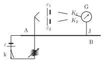
Method I -- connecting the cells individually. A potentiometer circuit is set up with a driving battery of emf , a key K and a rheostat across the wire AB, wired so that A is at higher potential than B. The two cells to be compared, of emf and , both have their POSITIVE terminals connected to point A, while their negative terminals go to the two outer terminals of a two-way key ; the central terminal of this key connects to a galvanometer, which in turn connects to a jockey touching the wire. With key K closed and closed (while stays open), only the first cell is in circuit with the galvanometer, and its null point is found at some length from A, so that
where k is the potential gradient of the wire. Then is opened and closed instead, bringing into the same circuit; its own null point is found at length from A, so that
Dividing the two equations cancels the (unknown) potential gradient k entirely, giving
so the two emfs can be compared purely from the two balancing LENGTHS -- and if either emf is independently known, the other follows immediately.
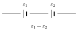
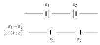
Method II -- the sum and difference method. When two cells are joined so the NEGATIVE terminal of the first meets the POSITIVE terminal of the second (exactly as cells are strung together in an ordinary battery), their emfs act in the same sense and add: the pair behaves as one effective source of emf -- this is called the SUM method (note that this is NOT the same thing as a parallel combination of cells). When instead the two cells are joined with their LIKE terminals together (both positive terminals tied together, or both negative terminals tied together), their emfs oppose and the pair behaves as one effective source of emf , taking as the larger of the two -- this is the DIFFERENCE method.
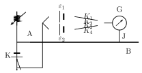
With both cells wired through four keys so that closing selects the sum configuration and closing selects the difference configuration, the SAME potentiometer wire and galvanometer are used to find a null point for each in turn. Let be the balancing length for the sum mode, so
and the balancing length for the difference mode, so
Dividing these two equations gives
and applying componendo-and-dividendo to this ratio isolates the emf ratio directly:
giving a second, independent way to compare the two emfs.
B) To find the internal resistance (r) of a cell
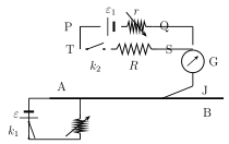
The set-up again uses a potentiometer wire AB in series with a driving cell of emf , a key and a rheostat, with A at higher potential than B. The cell whose internal resistance is to be found (its own emf ) is connected to the potentiometer wire through a galvanometer G and jockey J, and a resistance box R is connected across this same cell through a second key .
With closed and open, the circuit is simply the driving cell , the test cell and the potentiometer wire; the null point gives a length corresponding to the FULL emf of the test cell:
Now both and are closed, bringing the resistance box R into the circuit as an external load on the test cell; some resistance R is set on the box, and the (new, shorter) null point gives a length . Since the test cell is now delivering current I through R (with r its own internal resistance), this second balance length corresponds only to the TERMINAL potential difference across the loaded cell, not its full emf:
Applying Kirchhoff's voltage law to the test cell's own loop, while , gives
and combining this with from above and solving for r gives the internal-resistance formula
used numerically in Ex. 9.6, where a 1.5 V cell's balance length shifts from 76.3 cm (open circuit) to 64.8 cm once loaded by a 9.5 \Omega resistor, giving an internal resistance of about 1.69 \Omega.
C) Applications of the potentiometer …
Drawn by us to help you understand the concept clearly, and verified to make sure it's accurate. For exams, practice from your textbook's own diagram.
What this figure shows. A potentiometer circuit set up with a driving battery of emf , a key K and a rheostat across wire AB, arranged so point A is at higher potential than point B. The two cells whose emfs, and , are to be compared are connected with their POSITIVE terminals both joined to point A, and their negative terminals each going to one of the two outer terminals of a two-way key ; the central terminal of this two-way key connects on to a galvanometer, whose other terminal ends in a jockey J that touches the wire. Only one of / is closed at a time, so only ONE of the two cells is ever actually in circuit with the galvanometer branch at once, letti …
Drawn by us to help you understand the concept clearly, and verified to make sure it's accurate. For exams, practice from your textbook's own diagram.
What this figure shows. Two cells, of emf and , connected so that the NEGATIVE terminal of the first cell joins directly to the POSITIVE terminal of the second cell (i.e. connected the same way round, terminal-to-opposite-terminal, exactly as cells are joined in an ordinary series battery). Because the two cells' emfs then act in the SAME sense around the loop, their effect adds: the combination behaves as a single effective source of emf , which is why this connection is called the sum method -- explicitly distinguished in the …
Drawn by us to help you understand the concept clearly, and verified to make sure it's accurate. For exams, practice from your textbook's own diagram.
What this figure shows. The same two cells, of emf (taken larger) and , but now connected so that their like terminals are joined together -- either both negative terminals tied to one common point or both positive terminals tied to one common point (opposite of the sum-method wiring). Because the two emfs now act in OPPOSING senses around the loop, their effect subtracts: the combination behaves as a single effective source of emf , which is wh …
Drawn by us to help you understand the concept clearly, and verified to make sure it's accurate. For exams, practice from your textbook's own diagram.
What this figure shows. A potentiometer circuit built around the sum/difference cell pairing of Figs. 9.8(a)/(b), with the two cells , wired through FOUR keys, , , and , arranged so that closing and together connects the cells in the SUM configuration (emf in circuit with the potentiometer wire AB, galvanometer and jockey), while closing and together (with , open) switches to the DIFFERENCE configuration (emf ) using the same wire and galvanometer branch, so that a null point corresponding to each combination can be found in turn …
Worked out. A cell of emf 1.5 V is connected to a potentiometer; with the cell's external circuit OPEN, the balance (null) point is at 76.3 cm along the wire, and with a 9.5 \Omega resistor connected across the cell's own terminals (i.e. the cell now delivering current through this known external resistance), the balance point shifts to 64.8 cm. Using the internal-resistance formula with cm, cm and , the internal resistance works out to . This is the book's own worked instance of the general Part-B derivation: the OPEN-circuit balance length is proportional to the cell's full emf, while the CLOSED-circuit (loaded) balance length is proportional only to the smaller terminal voltage once some of the emf is dropped across the cell's own internal resistance, …
Drawn by us to help you understand the concept clearly, and verified to make sure it's accurate. For exams, practice from your textbook's own diagram.
This circuit determines the internal resistance r of a cell by the potentiometer method. The cell of emf ε₁ whose internal resistance is to be found is connected across the potentiometer wire AB through a galvanometer G and jockey J; a resistance box R with key k₂ can be connected across the cell. A driving cell ε with key k₁ and a rheostat sends a steady current through AB. With k₂ open, the balancing length l₁ corresponds to the emf ε₁; with k₂ closed and resistance R in circuit, the balancing length l₂ corresponds to the terminal volta …
Drawn by us to help you understand the concept clearly, and verified to make sure it's accurate. For exams, practice from your textbook's own diagram.
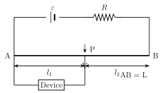
The potentiometer can act as a voltage divider that continuously varies the output voltage of a supply. A potential V is set up between the ends A and B of the potentiometer wire using a cell ε and series resistor R. A device is connected between the positive end A and a sliding contact P on the wire. As the slider moves, the output voltage divides in the ratio of the lengths l₁ (between A and P) and l₂ (between P and B), where AB = L. The output across the device is V₁ = (dV/dL)·l₁ …