Mathematics · Ch 9 — Applications of Integration
Area of the Region Bounded by a Curve, x-axis and the Lines x=a, x=b
Area of the Region Bounded by a Curve, x-axis and the Lines x=a, x=b
Case (i): curve above the -axis. Let , , be a continuous curve lying entirely above the -axis (in the first or second quadrant) between and , so throughout. Viewing the region bounded by the curve, the -axis, and the ordinates in the positive -direction, divide it into thin vertical strips of height and width . The area is the limit of the sum of the strip areas:
Case (ii): curve below the -axis. If lies entirely below the -axis (third/fourth quadrant) on , so throughout, each strip has height (a positive length), giving
Case (iii): curve crosses the -axis. If takes both signs on , divide at the crossing points into subintervals where keeps a constant sign, apply Cases (i)/(ii) on each piece, and add the (positive) areas:
…
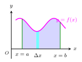
Drawn by us to help you understand the concept clearly, and verified to make sure it's accurate. For exams, practice from your textbook's own diagram.
What this figure shows. Fig. 9.8 — Area of the region bounded by a curve (above the x-axis), the x-axis and the ordinates , , built from vertical strips of …
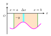
Drawn by us to help you understand the concept clearly, and verified to make sure it's accurate. For exams, practice from your textbook's own diagram.
What this figure shows. Fig. 9.9 — Area of the region bounded by a curve that lies below the x-axis, the x-axis and the ordinates , ; strip h …
![Fig. 9.10 — Fig. 9.10 — A curve $y=f(x)$ lying alternately above and below the x-axis on $[a,b]$, with geometric areas $A_1$, $A_2$, $A_3$, $A_4$ separated by $c_1$, $c_2$](/figures/applications-of-integration/area-four-regions-sine-curve-fig-9-10.svg)
Drawn by us to help you understand the concept clearly, and verified to make sure it's accurate. For exams, practice from your textbook's own diagram.
What this figure shows. Fig. 9.10 — A curve lying alternately above and below the x-axis on , with geometric areas , , , separated b …