Skip to content

Mathematics · Ch 3 — Trigonometric Functions

Inverse Sine Function

3.3.1

Inverse Sine Function

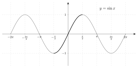
Consider sin⁡\sin restricted to [−π2,π2]→[−1,1]\left[-\dfrac{\pi}{2},\dfrac{\pi}{2}\right]\to[-1,1]. Graphically this restriction is one-one (strictly increasing) and onto [−1,1][-1,1], so its inverse exists, called the inverse sine function and denoted sin⁡−1:[−1,1]→[−π2,π2]\sin^{-1}:[-1,1]\to\left[-\dfrac{\pi}{2},\dfrac{\pi}{2}\right]. For x∈[−1,1]x\in[-1,1] and θ∈[−π2,π2]\theta\in\left[-\dfrac{\pi}{2},\dfrac{\pi}{2}\right], we write sin⁡−1x=θ\sin^{-1}x=\theta if sin⁡θ=x\sin\theta=x; θ\theta is called the principal value of sin⁡−1x\sin^{-1}x.

Ex.1 sin⁡π6=12\sin\dfrac{\pi}{6}=\dfrac12, where 12∈[−1,1]\dfrac12\in[-1,1] and π6∈[−π2,π2]\dfrac{\pi}{6}\in\left[-\dfrac{\pi}{2},\dfrac{\pi}{2}\right], so sin⁡−112=π6\sin^{-1}\dfrac12=\dfrac{\pi}{6}: the principal value of sin⁡−112\sin^{-1}\dfrac12 is π6\dfrac{\pi}{6}. Although sin⁡5π6=12\sin\dfrac{5\pi}{6}=\dfrac12 also, we cannot write sin⁡−112=5π6\sin^{-1}\dfrac12=\dfrac{5\pi}{6}, since 5π6∉[−π2,π2]\dfrac{5\pi}{6}\notin\left[-\dfrac{\pi}{2},\dfrac{\pi}{2}\right].

Ex.2 sin⁡(−π4)=−12\sin\left(-\dfrac{\pi}{4}\right)=-\dfrac{1}{\sqrt2}, where −12∈[−1,1]-\dfrac{1}{\sqrt2}\in[-1,1] and −π4∈[−π2,π2]-\dfrac{\pi}{4}\in\left[-\dfrac{\pi}{2},\dfrac{\pi}{2}\right], so sin⁡−1(−12)=−π4\sin^{-1}\left(-\dfrac{1}{\sqrt2}\right)=-\dfrac{\pi}{4}: the principal value of sin⁡−1(−12)\sin^{-1}\left(-\dfrac{1}{\sqrt2}\right) is −π4-\dfrac{\pi}{4}. …

Figure 3.8(a)Fig. 3.8(a) — Graph of y = sin x drawn over a wide domain, with its one-one restricted domain highlighted in bold
Fig. 3.8(a) — Fig. 3.8(a) — Graph of y = sin x drawn over a wide domain, with its one-one restricted domain highlighted in bold

Drawn by us to help you understand the concept clearly, and verified to make sure it's accurate. For exams, practice from your textbook's own diagram.

What this figure shows. Shows the graph of y=sin⁡xy=\sin x drawn only over the restricted interval [−π/2,π/2]\left[-\pi/2,\pi/2\right] on the x-axis, rising smoothly from −1-1 at x=−π/2x=-\pi/2 through the origin to +1+1 at x=π/2x=\pi/2, visually demonstrating that on this interval the curve is strictly increasing (one-one) and covers all of [−1,1][-1,1] (onto), which is exactly why an inverse can …
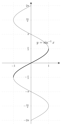
Figure 3.8(b)Fig. 3.8(b) — Graph of the inverse function y = sin⁻¹ x (reflection across y = x), with the principal branch in bold
Fig. 3.8(b) — Fig. 3.8(b) — Graph of the inverse function y = sin⁻¹ x (reflection across y = x), with the principal branch in bold

Drawn by us to help you understand the concept clearly, and verified to make sure it's accurate. For exams, practice from your textbook's own diagram.

What this figure shows. Shows the graph of y=sin⁡−1xy=\sin^{-1}x over its domain [−1,1][-1,1] on the x-axis, obtained by reflecting the restricted sine graph in the line y=xy=x; the curve rises from −π/2-\pi/2 at x=−1x=-1 through the origin to π/2\pi/2 at x=1x=1, confirming the stated range [−π/2,π/2]\left[-\pi/2,\pi/2\right] of the princi …