Parallel Resonance Circuit

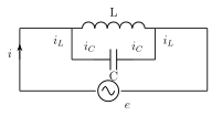
Now consider an inductor L and a capacitor C connected instead in PARALLEL with each other (Fig. 13.19), this combination connected across the AC source $e=e_0\sin\omega t$. Because they are in parallel, the SAME instantaneous voltage e appears across both branches, but the current in each branch is separately determined by that branch's own reactance and its own phase relationship: the inductor branch carries $i_L=\dfrac{e_0}{X_L}\sin\left(\omega t-\dfrac{\pi}{2}\right)$ (lagging), while the capacitor branch carries $i_C=\dfrac{e_0}{X_C}\sin\left(\omega t+\dfrac{\pi}{2}\right)$ (leading). Adding these two branch currents (they are $180^\circ$ out of phase with each other, since one lags by $\pi/2$ and the other leads by $\pi/2$) and simplifying using standard trigonometric identities gives the TOTAL current drawn from the source as $i=e_0\cos\omega t\left(\dfrac{1}{X_C}-\dfrac{1}{X_L}\right)$.

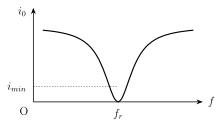
This total current is MINIMUM (in fact, ideally zero for a perfectly ideal, resistance-free L and C) exactly when $\dfrac{1}{X_C}=\dfrac{1}{X_L}$, i.e. when $X_L=X_C$ -- the SAME condition, $\omega=1/\sqrt{LC}$ or $f_r=\dfrac{1}{2\pi\sqrt{LC}}$, as for the series case, even though the circuit topology (and the direction of the effect on current) is entirely different. At this parallel resonant frequency, the individual branch currents $i_L$ and $i_C$ are each still very much present and can even be large, but being exactly opposite in phase, they cancel each other almost completely as seen from the source terminals -- so the TOTAL current drawn from the source is minimum, and correspondingly the impedance presented to the source is MAXIMUM, exactly the opposite behaviour to the series case (Fig. 13.20 shows the current dipping to a sharp minimum right at $f_r$, the mirror image of the series resonance curve's sharp peak). …