Series Resonance Circuit

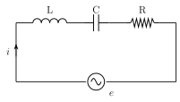
In a series LCR circuit (Fig. 13.17), the impedance is $Z=\sqrt{R^2+(X_L-X_C)^2}=\sqrt{R^2+\left(\omega L-\dfrac{1}{\omega C}\right)^2}$. At very low frequencies, $X_L=\omega L$ is small (negligible) while $X_C=1/(\omega C)$ is very large, so Z is large and dominated by the capacitor. As the frequency is increased, $X_L$ steadily grows while $X_C$ steadily shrinks, so at some particular angular frequency $\omega_r$ the two become exactly equal: $\omega_r L=\dfrac{1}{\omega_r C}$, which rearranges to $\omega_r=\dfrac{1}{\sqrt{LC}}$, or equivalently, in terms of ordinary frequency, $f_r=\dfrac{1}{2\pi\sqrt{LC}}$ -- the RESONANT FREQUENCY of the series LCR circuit.

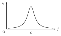
At exactly this frequency, the reactive term $(X_L-X_C)$ in the impedance formula vanishes, leaving $Z=\sqrt{R^2+0}=R$ -- the LEAST possible value the impedance can take (since the reactive term can never make a NEGATIVE contribution to $Z^2$, this is indeed the minimum). With impedance at its minimum, the current $i_0=e_0/Z=e_0/R$ is correspondingly at its MAXIMUM, and since $X_L=X_C$ means $\tan\phi=0$, voltage and current are exactly in phase (the circuit behaves as though it were purely resistive) at this frequency -- this combination of conditions (minimum impedance, purely resistive, maximum current) IS the resonance condition, and this particular frequency is called the series resonant frequency. The graph of rms current against frequency (Fig. 13.18, the 'series resonance curve') accordingly shows a single sharp peak exactly at $f_r$, low current well away from resonance on either side. …