Physics · Ch 14 — Dual Nature of Radiation and Matter

Observations from Experiments on Photoelectric Effect

14.2.2

Observations from Experiments on Photoelectric Effect

Careful experiments with the apparatus of the previous section, carried out over several decades, established a set of very specific facts about the photoelectric effect. Together they form the puzzle that classical (wave) theory could not solve, and that Einstein's photon picture would later explain completely.

First, a photocurrent appears ONLY if the frequency of the incident radiation exceeds some THRESHOLD FREQUENCY $\nu_0$ , which is fixed for a given metal but differs from one metal to another. If the frequency $\nu$ is above $\nu_0$ , electrons are emitted NO MATTER HOW FEEBLE the incident light is -- however small its intensity, some current always flows.

Second, there is essentially NO TIME LAG between the light being switched on and the photocurrent appearing: emission starts within about $10^{-9}$ s of illumination, even at very low intensity, and stops instantly the moment the light is switched off.

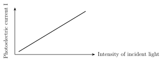
Third, for a fixed frequency (above threshold) and a fixed accelerating potential, the photocurrent I increases LINEARLY with the intensity of the incident radiation -- doubling the intensity exactly doubles the current, as shown by the straight-line graph through the origin in Fig. 14.3.

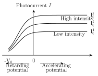
Fourth, the photocurrent also depends on the accelerating potential V itself. Starting from V = 0 and increasing V, the current I first rises, then LEVELS OFF at a constant value called the SATURATION CURRENT $I_0$ (Fig. 14.4) -- beyond a certain accelerating potential, every photoelectron ejected from E is already reaching C, so raising V further cannot increase the current any more.

Fifth, keeping the accelerating potential and frequency fixed, increasing the intensity increases the saturation current PROPORTIONATELY -- doubling the intensity doubles the saturation current, exactly mirroring the linear relationship of the third observation.

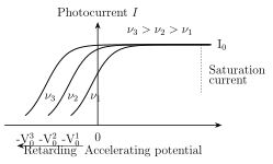
Sixth, and most striking of all: the MAXIMUM kinetic energy $KE_{max}$ of the emitted electrons depends on the FREQUENCY of the incident light and on the emitter material, but is COMPLETELY INDEPENDENT of the intensity. Changing the intensity (even making it very small) leaves $KE_{max}$ unchanged for a fixed frequency; only changing the frequency (or the metal) changes $KE_{max}$ .

Seventh, applying an increasingly NEGATIVE (retarding) potential to the collector causes the photocurrent to fall, until at some particular negative potential $-V_0$ it drops to exactly zero. This critical value $V_0$ is called the STOPPING POTENTIAL or CUT-OFF POTENTIAL: it is the minimum retarding potential needed to stop even the most energetic photoelectrons from reaching the collector. Crucially, $V_0$ stays the SAME regardless of the intensity of the incident light (Fig. 14.4), for a fixed frequency, but it DOES depend on the emitter material. …

Figure 14.3Fig. 14.3: Photocurrent as a function of incident intensity

Fig. 14.3 — Fig. 14.3: Photocurrent as a function of incident intensity

Drawn by us to help you understand the concept clearly, and verified to make sure it's accurate. For exams, practice from your textbook's own diagram.

What this figure shows. A graph with the horizontal axis showing the intensity of incident radiation and the vertical axis showing photocurrent I, plotted for a FIXED incident frequency and a fixed (positive, accelerating) potential V between emitter and collector. The plotted curve is a straight line passing through the origin, rising with a constant positive slope -- showing that, once frequency and accelerating potential are held fixed, the photocurrent increases exactly linearly (proportionally) with the intensity of the incident light, with no saturation or bendin …

Figure 14.4Fig. 14.4: Photocurrent vs accelerating potential for fixed frequency, different intensities

Fig. 14.4 — Fig. 14.4: Photocurrent vs accelerating potential for fixed frequency, different intensities

Drawn by us to help you understand the concept clearly, and verified to make sure it's accurate. For exams, practice from your textbook's own diagram.

What this figure shows. A graph with accelerating potential V on the horizontal axis (extending to both positive and negative values, i.e. including the retarding-potential region) and photocurrent I on the vertical axis, for a FIXED incident frequency but several different incident intensities, plotted as a family of curves labelled with superscripts 1, 2, 3 corresponding to increasing intensity. Each curve rises steeply from the negative-V (retarding) side, crosses zero current at the SAME negative potential -V0 (the stopping potential, identical for all three curves since frequency is fixed), then increases with increasing positive V before flattening out to its own distinct horizontal plateau -- the saturation current $I_0^{1}<I_0^{2}<I_0^{3}$ -- with the highest-intensity curve saturating at the highest current. The figure's key point is that all three curves share exactly the same stopping potential -V0 bu …

Figure 14.5Fig. 14.5: Photocurrent vs accelerating potential for fixed intensity, different frequencies

Fig. 14.5 — Fig. 14.5: Photocurrent vs accelerating potential for fixed intensity, different frequencies

Drawn by us to help you understand the concept clearly, and verified to make sure it's accurate. For exams, practice from your textbook's own diagram.

What this figure shows. A graph with accelerating potential V (including negative, retarding values) on the horizontal axis and photocurrent I on the vertical axis, for a FIXED incident intensity but three different incident frequencies $\nu_1<\nu_2<\nu_3$ (labelled directly on the three curves), all for the SAME emitter material. All three curves rise to and level off at the SAME saturation current value (since intensity, and hence the number of incident photons per second, is held fixed), but each crosses zero current at a DIFFERENT, more negative stopping potential as frequency increases -- so the curve for $\nu_3$ (the highest frequency) cuts the horizontal axis furthest to the left (most negative V), followed by $\nu_2$ , then $\nu_1$ closest to the origin. This shows that increasing frequency increases the stopping potential (hence the maximum photoelectron kinetic e …

Start your 14-day free trial to unlock the full solution →

← Previous · 14.2.1Experimental Set-up of Photoelectric Effect Next · 14.2.3 →Failure of Wave Theory to Explain the Observations from Experiments on Photoelectric Effect