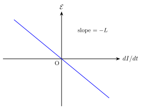
Draw the graph showing variation of the value of the induced emf as a function of rate of change of current fl

Question

Q. Draw the graph showing variation of the value of the induced emf as a function of rate of change of current flowing through an ideal inductor.

CBSECBSE Class XII Board 2020Subjective· 1mImportance★★★★★

🔒 Locked · start free trial →

You're viewing a preview — the full solution, concept, methods & PYQ mapping are locked.

Start your 14-day free trial to unlock the full solution →

Concept understanding — Self-Inductance of a Solenoid

Self-Inductance of a Solenoid: From Intuition to Formula

Imagine you push a heavy door. It doesn't resist your push once it's moving — but it does resist you trying to change its speed suddenly. That resistance to change is inertia. A solenoid carrying current behaves the same way: it "wants" to keep its current steady, and fights any attempt to change it.

This property is called self-inductance. The solenoid generates a back emf that opposes the change in its own current — not the current itself, but the change in current. That's the core idea.

Why does a solenoid oppose current changes?

A solenoid is a long coil of wire. When current flows through it, it produces a magnetic field inside. If you try to increase the current, the magnetic field strengthens. But a changing magnetic field induces an emf in the coil itself (Faraday's law). By Lenz's law, this induced emf opposes the change that caused it — so it pushes back against the rising current.

If you try to decrease the current, the field weakens, and the induced emf tries to keep the current flowing. The solenoid acts like an electrical "flywheel."

The precise statement

Self-inductance $L$ is defined by the relation:

\mathcal{E} = -L \frac{dI}{dt}

where $\mathcal{E}$ is the induced back emf, and $\frac{dI}{dt}$ is the rate of change of current. The negative sign tells you the emf opposes the change.

For a solenoid, $L$ depends only on its geometry and the core material — not on the current. The formula is:

L = \mu_0 n^2 A l

L = \mu_0 n^2 A l

Let's unpack each symbol:

$\mu_0$ — permeability of free space ( $4\pi \times 10^{-7}$ H/m). It's a universal constant that tells you how strongly a vacuum responds to magnetic fields.
$n$ — number of turns per unit length (turns/m). More turns per metre means a stronger field per ampere, so more inductance.
$A$ — cross-sectional area of the solenoid (m²). A wider coil encloses more magnetic flux.
$l$ — length of the solenoid (m). Longer solenoid means more total turns, hence more inductance.

Where does $L = \mu_0 n^2 A l$ come from?

Start with the magnetic field inside a long solenoid:

B = \mu_0 n I

The magnetic flux through one turn is $BA = \mu_0 n I A$ . For all $N = nl$ turns, the total flux linkage is:

\Phi_{\text{total}} = N \cdot BA = (nl)(\mu_0 n I A) = \mu_0 n^2 A l I

By definition, self-inductance is the constant of proportionality between flux linkage and current:

\Phi_{\text{total}} = L I

Comparing, you get:

L = \mu_0 n^2 A l

Note

This formula assumes an ideal solenoid — infinitely long, with a uniform field inside and zero field outside. Real solenoids are close approximations if $l \gg \sqrt{A}$ .

What does a larger $L$ mean?

A solenoid with high $L$ strongly resists changes in current. If you try to switch the current on quickly, the back emf is large, so the current rises slowly. If you short-circuit the solenoid, the current doesn't drop instantly — it decays gradually.

This is why inductors are used in filters, chokes, and timing circuits. They smooth out current variations. …

Start your 14-day free trial to unlock the full solution →

For an ideal inductor, the induced emf is directly proportional to the rate of change of current, given by $\mathcal{E} = -L \frac{dI}{dt}$ . The graph is a straight line through the origin with slope $-L$ .

Graph of induced emf versus the rate of change of current for an ideal inductor: a straight line through the origin with negative slope -L, so that the induced emf E = -L(dI/dt) is positive when the current is decreasing and negative when the current is increasing.

The Concept: Why This Relationship Exists

An ideal inductor is a coil of wire with zero resistance. When current changes through it, the magnetic flux linked with the coil changes. By Faraday's law, this changing flux induces an emf that opposes the change — that's Lenz's law at work.

The key insight: the induced emf doesn't depend on how much current is flowing, but on how fast the current is changing. A steady current produces no induced emf at all. This is why the graph relates $\mathcal{E}$ to $\frac{dI}{dt}$ , not to $I$ itself.

\mathcal{E} = -L \frac{dI}{dt}

Step-by-Step Reasoning

1. Identify the independent and dependent variables

The question asks for induced emf as a function of the rate of change of current. So:

Horizontal axis: $\frac{dI}{dt}$ (rate of change of current)
Vertical axis: $\mathcal{E}$ (induced emf)

2. Apply the defining equation for an ideal inductor

For an ideal inductor (no internal resistance), the relationship is exactly:

\mathcal{E} = -L \frac{dI}{dt}

This is a linear equation of the form $y = mx$ , where:

$y = \mathcal{E}$
$x = \frac{dI}{dt}$
$m = -L$ (the slope)

3. Interpret the slope

Since $L$ is a positive constant (inductance is always positive), the slope $-L$ is negative. This means:

When $\frac{dI}{dt} > 0$ (current increasing), $\mathcal{E} < 0$ (emf opposes the increase)
When $\frac{dI}{dt} < 0$ (current decreasing), $\mathcal{E} > 0$ (emf opposes the decrease)
When $\frac{dI}{dt} = 0$ (steady current), $\mathcal{E} = 0$

Watch out

A common mistake is to draw the graph with positive slope, forgetting the negative sign from Lenz's law. The induced emf always opposes the change, so the slope must be negative.

4. Determine the graph's shape

The equation $\mathcal{E} = -L \frac{dI}{dt}$ is a straight line passing through the origin. No curvature, no intercept — just a straight line with negative slope.

5. Consider the range of values

The rate of change of current can be positive, negative, or zero. So the graph extends into both quadrants:

First quadrant: $\frac{dI}{dt} > 0$ , $\mathcal{E} < 0$ (below the horizontal axis) …

Start your 14-day free trial to unlock the full solution →

Same / Similar Concept — real previous-year questions on the same or a closely similar concept, not this exact question.

Showing the 12 most recent of 35 on this concept.

CBSE 2026Set ANNUAL1 markMCQ
$Q. When the current changes from +2 A to -2 A in 0.05 second in a coil, an e.m.f. of 8 V is induced in it. The coefficient of self-induction of the coil is$
(a) 0.1 henry
(b) 0.2 henry
(c) 0.4 henry
(d) 0.8 henry
›Reveal solutionSolution

Using $e = L\,\Delta I/\Delta t$ with $\Delta I = 4$ A and $\Delta t = 0.05$ s gives $L = 0.1$ H.

The current changes from $+2$ A to $-2$ A, so the magnitude of the change is

$\Delta I = |(-2) - (2)| = 4\ \text{A}, \qquad \Delta t = 0.05\ \text{s}$

The magnitude of the self-induced emf is …

Start your 14-day free trial to see the full solution →
CBSE 2026Set ANNUAL1 markMCQ
$Q. Self inductance is called$
(a) electric force
(b) electrical inertia
(c) electric pressure
(d) electric energy
›Reveal solutionSolution

Self-inductance L makes a circuit resist a change in the current flowing through it (via a back-emf = -L dI/dt), analogous to inertia resisting a change in velocity.

Whenever the current through a coil tends to change, the induced back-emf (from self-induction) opposes that change (Lenz's law). This behaviour - opposing change rather than opposing the current itself - is directly analogous to mechanical inertia, which oppos …

Start your 14-day free trial to see the full solution →
CBSE 2026Set ANNUAL1 markMCQ
$Q. The self-inductance of a coil is measured by$
(a) Electrical inertia
(b) Electrical friction
(c) Induced emf
(d) Induced current
›Reveal solutionSolution

Self-inductance is defined via the induced emf a coil produces in itself when its own current changes - it behaves like the 'electrical inertia' of the circuit, but it is quantified through that induced emf.

When the current I through a coil changes, the magnetic flux linked with the coil changes too, and by Faraday's law this changing self-flux induces an emf in the SAME coil that opposes the change in current (Lenz's law). This self-induced emf defines the self-inductance L of the coil:

emf = -L * (dI/dt)

…

Start your 14-day free trial to see the full solution →
CBSE 2026Set ANNUAL1 markMCQ
$Q. The unit of inductance is$
(a) henry
(b) weber
(c) newton
(d) ohm
›Reveal solutionSolution

Inductance L relates induced emf to the rate of change of current, so its unit works out to volt-second per ampere - named the henry.

From emf = -L*(dI/dt), we get L = emf / (dI/dt), so the unit of L is volt / (ampere/second) = volt.second/ampere. This combination is given the special SI name henry (H), after Joseph Henry. Weber is the u …

Start your 14-day free trial to see the full solution →
CBSE 2026Set ANNUAL1 markMCQ
$Q. In a solenoid number of turns per unit length are doubled, it's self-inductance:$
(a) Halved
(b) Doubled
(c) Remains constant
(d) Becomes four times
›Reveal solutionSolution

Self-inductance of a solenoid is proportional to the square of the number of turns per unit length, so doubling $n$ makes $L$ four times as large.

…

Start your 14-day free trial to see the full solution →
CBSE 2026Set ANNUAL1 markMCQ
$Q. Current in a circuit falls from 5.0 A to 0.0 A in 0.1 s. If an average e.m.f. of 100 V induced, give an estimate of the self-inductance of the circuit.$
(a) L = 4 H
(b) L = 20 H
(c) L = 40 H
(d) L = 2 H
›Reveal solutionSolution

Using $|\varepsilon| = L\left|\dfrac{dI}{dt}\right|$ , the self-inductance works out to 2 H.

Given: Current changes from $I_i = 5.0\text{ A}$ to $I_f = 0.0\text{ A}$ in $\Delta t = 0.1\text{ s}$ , with average induced emf $|\varepsilon| = 100\text{ V}$ .

Step 1 — rate of change of current:

$\left|\frac{\Delta I}{\Delta t}\right| = \frac{5.0 - 0.0}{0.1} = 50\ \text{A/s}$

…

Start your 14-day free trial to see the full solution →
CBSE 2025Set X11 mark
$Q. When a ________ rod is inserted into a coil, its self-inductance increases.$
›Reveal solutionSolution

ferromagnetic (soft iron) Self-inductance $L = \mu_r \mu_0 n^2 A l$ . Inserting a ferromagnetic (soft iron) core has a large relative permeability $\mu_r \gg 1$ , which greatly increases the mag …

Start your 14-day free trial to see the full solution →
CBSE 2025Set D1 markMCQ
$Q. The self-inductance of a solenoid depends on (A) The current flowing through its medium (B) The number of turns per unit length (C) The length of the solenoid (D) Both (B) and (C)$
›Reveal solutionSolution

Self-inductance depends on the solenoid's geometry (turns per unit length and length/area), not on the current.

For a solenoid the self-inductance is

$L = \mu_0 n^{2} A l$

where n is the number of turns per unit length, A the cross-sectional area and l the length. So it depends on the number of turns per unit length and the length (and area) — both geometric factors.

…

Start your 14-day free trial to see the full solution →
CBSE 2025Set ANNUAL1 markMCQ
$Q. The self-inductance of a coil is 5 henry. A current of 1 ampere changes to 2 amperes within 5 seconds through the coil. The value of the induced e.m.f. is$
(i) 10 volts
(ii) 0.1 volt
(iii) 1 volt
(iv) 100 volts
›Reveal solutionSolution

emf = L dI/dt = 5 x (1 A / 5 s) = 1 V.

…

Start your 14-day free trial to see the full solution →
CBSE 2024Set A11 markMCQ
$Q. Current in a coil changes from 1.6 A to 0.2 A in 2 second inducing an emf of 2.8 V. The value of self-inductance of the coil is$
(a) 40 H
(b) 28 H
(c) 4 H
(d) 56 H
›Reveal solutionSolution

(c) 4 H …

Start your 14-day free trial to see the full solution →
CBSE 2024Set A1 markMCQ
$Q. S.I. unit of self-induction is (A) coulomb (C) (B) volt (V) (C) ohm (Ω) (D) henry (H)$
›Reveal solutionSolution

The SI unit of self-inductance L is the henry (H).

Self-inductance L links the flux (or back-emf) of a coil to the current through it:

$\phi = LI \qquad\text{and}\qquad \varepsilon = -L\frac{dI}{dt}.$

…

Start your 14-day free trial to see the full solution →
CBSE 2024Set ANNUAL1 markMCQ
$Q. The SI unit of self-inductance of a coil is$
(a) farad
(b) henry
(c) weber
(d) oersted
›Reveal solutionSolution

Self-inductance L is defined by the induced EMF equation EMF = −L(dI/dt); its SI unit is the henry (H).

When the current through a coil changes, the changing magnetic flux linked with the coil itself induces an EMF in it (self-induction). This is written as:

EMF = −L (dI/dt)

where L is the coefficient of self-inductance of the coil. Rearranging, L = −EMF/(dI/dt), so the unit of L is volt/(ampere/second) = volt·second/ampere. This combination is given the special SI name henry (H), where 1 H = 1 V·s/A.

…

Start your 14-day free trial to see the full solution →

Q.Draw the graph showing variation of the value of the induced emf as a function of rate of change of current flowing through an ideal inductor.

The Concept: Why This Relationship Exists

Step-by-Step Reasoning

🎓Unlock everything free for 14 days

Unlock everything free for 14 days