Physics · Ch 8 — Electrostatics

Equipotential Surfaces

8.5

Equipotential Surfaces

An EQUIPOTENTIAL SURFACE is a surface on which the electric potential has the identical value at every single point. For a single point charge $q$ , since $V=\dfrac{1}{4\pi\epsilon_0}\dfrac{q}{r}$ depends on $r$ alone, every sphere of a fixed radius centred on the charge is one equipotential surface -- so the full family of equipotential surfaces around an isolated point charge is a set of CONCENTRIC SPHERES, closer together near the charge (where $V$ changes rapidly with distance) and progressively farther apart at greater distances (where $V$ changes more slowly). For an infinite line charge, by contrast, the matching family of equipotential surfaces is a set of coaxial CYLINDERS rather than spheres, since the underlying symmetry is cylindrical rather than spherical.

Two points P and Q on the SAME equipotential surface, by definition, share $V_P=V_Q$ . Since the potential difference between any two points equals the work done per unit charge moving between them, $V_P-V_Q=W_{QP}$ , it follows immediately that $W_{QP}=0$ -- moving a test charge between any two points on one equipotential surface costs NO net work at all, however far apart those two points actually are along the surface.

This zero-work property forces a deep geometric fact about the field. Consider a small displacement $dx$ taken ALONG the equipotential surface itself: the work done is $dW=q_0E\,dx\cos\theta$ , where $\theta$ is the angle between $\vec{E}$ and the displacement. Since this work must be exactly zero for EVERY such displacement along the surface (not just some), and $E$ itself is not generally zero, the only way to guarantee $dW=0$ for arbitrary in-surface displacements is $\cos\theta=0$ , i.e. $\theta=90^\circ$ : the electric field must be exactly NORMAL (perpendicular) to the equipotential surface at every single point, for ANY charge distribution whatsoever, not merely for the simple symmetric cases. The converse argument makes the same point from the other direction: were the field to have ANY non-zero component lying along the surface, moving a charge against that in-surface component would require work -- directly contradicting the surface's own defining zero-potential-difference property.

A direct and important consequence: two DIFFERENT equipotential surfaces (at two different potential values) can NEVER intersect one another. If they did, the point of intersection would have to lie simultaneously on both surfaces -- meaning the field there would have to be normal to two different surface orientations at once, i.e. point in two different directions simultaneously, which is physically impossible for a single, well-defined field vector at one point. …

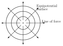
Figure 8.10Fig. 8.10: Equipotential surfaces (general)

Fig. 8.10 — Fig. 8.10: Equipotential surfaces (general)

Drawn by us to help you understand the concept clearly, and verified to make sure it's accurate. For exams, practice from your textbook's own diagram.

What this figure shows. A family of concentric circles (the cross-section of concentric spheres) drawn around a central point charge, each circle representing one equipotential surface at a different, labelled potential value, with the circles spaced closer together near the charge (where $V$ changes rapidly with $r$ ) and progressively farther apart at greater distances (where $V$ changes more slowly) -- the basic picture of concentric-sphere equipotentials for an isolated point charge intro …

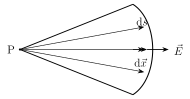
Figure 8.11Fig. 8.11: Equipotential surface and the normal field vector E

Fig. 8.11 — Fig. 8.11: Equipotential surface and the normal field vector E

Drawn by us to help you understand the concept clearly, and verified to make sure it's accurate. For exams, practice from your textbook's own diagram.

What this figure shows. A single curved equipotential surface with a point marked on it, and the field vector $\vec{E}$ drawn as an arrow at that point, exactly perpendicular (normal) to the surface at the point of contact -- with a small displacement $dx$ ALONG the surface (at angle $\theta=90^\circ$ to $E$ ) also indicated, visually justifying why $E\,dx\cos90^\circ=0$ , i.e. the work done moving a charge along this surface element is zero, and hence why the field must be normal to any equipotential surfa …

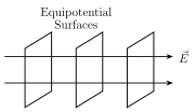
Figure 8.12Fig. 8.12: Equipotential surfaces for a uniform electric field

Fig. 8.12 — Fig. 8.12: Equipotential surfaces for a uniform electric field

Drawn by us to help you understand the concept clearly, and verified to make sure it's accurate. For exams, practice from your textbook's own diagram.

What this figure shows. A region of uniform electric field (parallel, equally-spaced field lines running in one fixed direction, such as between two charged parallel plates), with a family of flat PLANES drawn perpendicular to those field lines, evenly spaced along the direction of the field -- each plane is one equipotential surface, and because the field is uniform, the planes are drawn EQUALLY spaced from each other, unlike the unevenly-spaced spheres of a point charge, reflecting that $V$ changes at a constant rate with dista …

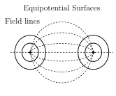
Figure 8.13Fig. 8.13: Equipotential surfaces for a dipole

Fig. 8.13 — Fig. 8.13: Equipotential surfaces for a dipole

Drawn by us to help you understand the concept clearly, and verified to make sure it's accurate. For exams, practice from your textbook's own diagram.

What this figure shows. A dipole (charges $-q$ and $+q$ separated by $2l$ ) with a set of closed, non-spherical, egg-shaped/distorted curves drawn around it representing its equipotential surfaces -- surfaces bunched closer and more tightly curved near each individual charge (where the local field is strongest and dominated by that one charge alone), and a single straight equipotential line/plane running through the exact midpoint of the dipole, perpendicular to its axis, at potential exactly zero -- this is the equatorial plane established algebraically in section 8.4.2, shown here as the flat boundary separating the positive-potential surfaces (near …

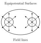
Figure 8.14Fig. 8.14: Equipotential surfaces for two identical positive charges

Fig. 8.14 — Fig. 8.14: Equipotential surfaces for two identical positive charges

Drawn by us to help you understand the concept clearly, and verified to make sure it's accurate. For exams, practice from your textbook's own diagram.

What this figure shows. Two equal positive point charges placed near each other, with a family of closed curves drawn around them representing their combined equipotential surfaces -- small, nearly circular closed curves tightly encircling each individual charge close in (where that one charge's own field dominates), which progressively merge into larger, single, dumbbell/peanut-shaped closed curves encircling BOTH charges together at greater distance (where the combined field of the pair becomes the dominant, symmetric far-field pattern) -- unlike the dipole's pattern, there is no zero-potential surface anywhere, since both charges contribute the SAME …

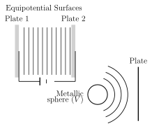
Figure 8.15Fig. 8.15 (a)-(b): Equipotential surfaces between plates, and plate-vs-sphere

Fig. 8.15 — Fig. 8.15 (a)-(b): Equipotential surfaces between plates, and plate-vs-sphere

Drawn by us to help you understand the concept clearly, and verified to make sure it's accurate. For exams, practice from your textbook's own diagram.

What this figure shows. Panel (a) shows two flat, parallel, oppositely-charged metallic plates with a family of evenly-spaced flat equipotential planes drawn in the uniform-field region between them, parallel to the plates themselves -- the same uniform-field picture as Fig. 8.12, specifically drawn for the two-plate geometry. Panel (b) shows one of the two plates REPLACED by a charged metallic SPHERE facing the other flat plate, with the equipotential surfaces now shown distorted -- flat and evenly spaced near the remaining flat plate, but curving to wrap around the spherical electrode's own curvature near it, illustrating that equipotential surfaces conform to the SHAPE of the nearby conductor that produces them, not to …

Misc Ex.9Example 8.9: A charged particle in equilibrium between two plates

Worked out. A particle of charge $q=1.6\times10^{-19}$ C (magnitude; negative) is suspended in equilibrium between two horizontal metal plates $dx=10\,\text{cm}=10^{-1}$ m apart, with potential difference $dV=4000$ V across them. The field between the plates is $E=\dfrac{dV}{dx}=\dfrac{4000}{10^{-1}}=4\times10^4\,\text{V m}^{-1}$ . For equilibrium, the electric force must exactly balance gravity: $F=mg=qE$ , so $m=\dfrac{qE}{g}=\dfrac{1.6\times10^{-19}\times4\times10^4}{9.8}\approx6.53\times10^{-16}$ kg -- an application of the uniform parallel-plate field formula $E=V/d$ to a force-balance problem, the same physical set-up (charged particle levitating in a uniform fi …

Start your 14-day free trial to unlock the full solution →

← Previous · 8.4.3Electric Potential due to a System of Charges Next · 8.6 →Electrostatic Potential Energy of Two Point Charges and of a Dipole in an Electrostatic Field