Physics · Ch 8 — Electrostatics
Electric Potential due to a System of Charges
Electric Potential due to a System of Charges
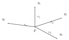
Now generalise from one or two source charges to N arbitrary point charges , sitting at respective distances from a common field point P. Each individual charge produces its own potential at P exactly as derived in section 8.4.1, , completely independently of every other charge present.
The crucial simplification compared to computing the FIELD due to many charges is that potential is a SCALAR, so the superposition principle here means an ordinary algebraic (signed) sum -- no components, no angles, no vector addition are needed at all: . This is often the most efficient route to a problem even when the FIELD is ultimately wanted, since it can be much easier to first sum up all the scalar potentials from every source charge and only afterward differentiate (using , section 8.3) to recover the field, rather than summing vector field contributions directly from the start. …
Drawn by us to help you understand the concept clearly, and verified to make sure it's accurate. For exams, practice from your textbook's own diagram.
What this figure shows. A field point P surrounded by several discrete point charges scattered at various positions, each joined to P by a line labelled with its own distance . No force or field arrows are drawn (unlike the corresponding superposition figure for fields) -- only the charges and their individual distances to P -- visually emphasising that computing the NET potential at P needs nothing more than these scalar distances and the individual charge mag …
Worked out. Charges C and C are 16 cm apart on the x-axis, with at the origin. Setting the sum of their potentials to zero at a point P, from the origin: for P between the charges gives, after simplifying, m -- a point 10 cm from (and hence 6 cm from ) where the larger-but-farther positive contribution exactly cancels the smaller-but-closer negative one. A second zero-potential point also exists OUTSIDE the segment, beyond on the far side (along the extended line, where 's closer negative contribution can still be cancelled by 's larger charge from farther away): solving the corresponding equation for that configuration gives m cm from the origin -- illustrating that a syste …