Electronics · Ch 8 — Modulation and Demodulation
Frequency modulation
Frequency modulation
Frequency modulation (FM) is a modulation system developed in 1936 as an alternative to AM. Amplitude modulation is not an efficient way to transmit voice and music, and it is vulnerable to noise. FM overcomes both weaknesses: it has strong resistance to noise (better noise immunity) and gives high-fidelity reproduction, which is why it is used at VHF for music and speech broadcasts. There is also a key difference in bandwidth behaviour — in AM the transmission bandwidth grows with the signal bandwidth, whereas in FM the transmission bandwidth is large but is essentially unaffected by the signal bandwidth.
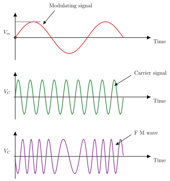
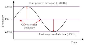
Frequency modulation is the process by which the frequency of the carrier is varied in accordance with the instantaneous amplitude of the modulating signal, while the carrier amplitude stays constant. When the modulating signal is zero, the carrier stays at its rest (centre) frequency ; a rising modulating amplitude raises the carrier frequency and a falling amplitude lowers it, with the maximum deviation occurring at the positive and negative peaks of the modulating signal (Figures 8.5.1 and 8.5.2).
Mathematical representation of FM
Let the modulating voltage be
and the carrier be
Writing the total instantaneous phase angle as (8.29) gives (8.30), with . During frequency modulation the carrier's angular frequency varies with time in step with the modulating voltage:
where is the modulation deviation constant, or frequency sensitivity of the modulator.
Frequency deviation and carrier swing
Dividing (8.31) by , the instantaneous carrier frequency is . It reaches its extremes when :
The frequency deviation (also written ) is the change of carrier frequency from its centre value produced by the modulating signal:
Importantly, the frequency deviation is independent of the modulating frequency and is proportional to the amplitude of the modulating signal. The carrier swing (CS) is the total variation from the minimum to the maximum frequency:
Integrating (8.31) and neglecting the constant of integration gives the phase
so the FM carrier voltage becomes
with .
Modulation index
The FM modulation index is the ratio of the maximum frequency deviation to the modulating-signal frequency:
It has no unit and is expressed as a decimal. For a fixed frequency deviation, decreases as the modulating frequency rises. The modulation index is what is used to calculate the bandwidth and the number of significant sidebands of an FM wave. (Unlike AM, can be much greater than 1.)
Deviation ratio
The deviation ratio describes the worst case of the modulation index — the ratio of the maximum allowed frequency deviation to the maximum frequency of the modulating signal:
It is widely quoted in FM broadcasting and TV: for FM broadcast it is , and for TV sound it is . It is used to find the worst-case bandwidth of a transmitter.
Percent modulation
In FM, percent modulation has a different meaning from AM. Because the modulating signal varies only the carrier frequency, percent modulation compares the actual carrier deviation with the maximum permitted deviation:
Broadcast FM
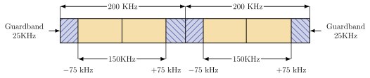
By FCC allocation the FM broadcast band runs from 88 to 108 MHz. Each station is allowed a deviation of kHz, so the FM channel bandwidth is kHz. A 25 kHz guard band is added on either side of the channel to prevent interference between adjacent stations, giving a total of 200 kHz per station (Figure 8.5.3). Commercial FM stations must follow these values: maximum frequency deviation kHz; carrier frequency stability kHz; maximum allowed audio frequency 15 kHz; guard band 50 kHz (25 kHz on each side); and maximum bandwidth 200 kHz per channel.
Frequency spectrum of FM
Unlike AM, an FM wave modulated by a single tone contains an infinite number of sidebands, whose amplitudes are given by Bessel functions of the first kind of the modulation index. The FM wave expands as
where are the zero-, first-, second-order Bessel coefficients, , and is the peak unmodulated carrier value.
The textbook prints this expansion without the brackets shown above, so it can read as though each multiplies only the first sine term. The official corrigendum corrects the first-order term to , and similarly for every other order — i.e. each Bessel coefficient multiplies both of its sideband terms. The corrected, bracketed form is used here.
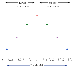
From this expansion we observe: (1) the first term is the carrier; (2) the FM wave contains infinitely many sidebands, each separated from the next by ; (3) the sidebands are distributed symmetrically about , so sidebands equidistant from the carrier have equal amplitudes; and (4) the amplitudes of the carrier and sidebands depend on the coefficients, which depend on the modulation index and are read from a standard Bessel table. Figure 8.5.4 shows the FM spectrum for particular values of and .
Significant sidebands
Although an FM wave has infinitely many sidebands, most are too small to matter. Significant sidebands are those whose amplitude is at least 1% of the carrier amplitude. Their number is fixed by the modulation index.
Bandwidth
The theoretical bandwidth of an FM wave is infinite, but in practice it is set by the number of significant sidebands. Bandwidth is defined as the width of the frequency spectrum containing all side frequencies with amplitude of the carrier. For significant sidebands,
A convenient estimate is Carson's rule — the bandwidth is twice the sum of the maximum frequency deviation and the highest modulating frequency:
FM modulators
An FM signal is generated with a device whose reactance can be varied by an applied voltage — a FET, a BJT or a varactor diode. If such a device is placed across the tank circuit of an oscillator, then varying its reactance with the modulating voltage varies the oscillator frequency and produces FM. Two common circuits are the varactor-diode modulator and the transistor reactance modulator.
Varactor diode modulator
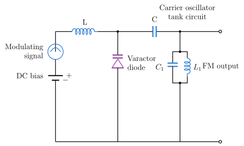
A varactor diode is a diode whose junction capacitance changes with the reverse voltage applied to it. In the varactor-diode modulator (Figure 8.5.5) the diode is connected across the oscillator tank circuit through a coupling capacitor C of relatively large value, which provides DC isolation between the oscillator and the diode; an RF choke L passes the low-frequency modulating signal but blocks the RF. Working: the modulating signal is applied in series with the DC bias; passing through the RF choke, it appears across the varactor diode and changes its capacitance in step with the modulating signal. This alters the total tank capacitance and hence the oscillator frequency, producing an FM wave. Being a simple two-terminal device, the varactor diode is also used for automatic frequency control and remote tuning.
Reactance modulator
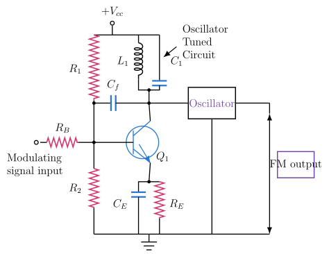
The transistor reactance modulator (Figure 8.5.6) is widely used for FM generation and gives better stability than the varactor circuit; it is used with a Hartley or Colpitts oscillator. A capacitor and resistor introduce a 90° phase shift between the collector voltage and current (the current leads the voltage by 90°), so the stage behaves like a voltage-controlled capacitor placed in parallel with the oscillator's tuned circuit. Working: the information signal applied to the base has the same effect as varying the transistor bias, which increases or decreases this voltage-controlled capacitance. That changes the effective capacitance of the tuned circuit and hence its resonance frequency, so the oscillator frequency varies with the modulating-signal amplitude and the output is an FM signal.
FM transmitter …
The process by which the frequency of the carrier is varied in accordance with the instantaneous amplitude of the modulating signal, while the carrier amplitude is kept constant. When the message is zero the carrier …
(8.34), where the modulation index . The carrier amplitude is constant; only the …
: the change in carrier frequency from its centre value caused by the modulating signal. It is independent of the modulating frequency and propo …
(8.32): the total frequency variation of the FM carrier, from its minimum to its maximum, equal to twice the frequency deviation. Here (also written ) is the frequency deviation, so the carrier swings the same amount above and below its centre frequency ; the carrier swing …
(8.35): the ratio of the maximum frequency deviation to the modulating-signal frequency. It has no unit, may be much greater than 1, and determines the bandwidth a …
Deviation ratio (8.36): maximum allowed deviation divided by the maximum modulating frequency. FM broadcast ; TV sound . It describes the worst case of the modulation index and is used to find the worst-cas …
(8.37): the ratio of the actual carrier deviation to the maximum permitted deviation, expressed as a percentage. Here is the actual deviation and the maximum permitted deviation. Unlike AM, it compares deviations rather than ampli …
For significant sidebands (8.38). Carson's rule estimates (8.39). Here is the modulating frequency, the peak deviation and the modulation index. Carson's rule gives a quick practical estimate of th …
The FM sidebands whose amplitude is at least 1% of the carrier amplitude. Only these are counted when finding the practical bandwidth; their number is set by the modulation index. Although an FM wave has infinitely many sidebands, most are too small to matter; only these significant ones are counted …
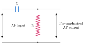
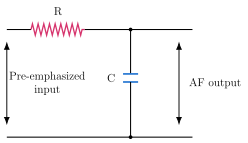
Pre-emphasis boosts the relative amplitudes of the higher-frequency components of the modulating signal (above ~1 kHz) at the transmitter, using an RC high-pass filter, to improve the signal-to-noise ratio; de-emphasis at the …
Drawn by us to help you understand the concept clearly, and verified to make sure it's accurate. For exams, practice from your textbook's own diagram.
Figure 8.5.1 (Principle of Frequency Modulation): three stacked waveforms — the low-frequency modulating sine (), the constant-amplitude carrier (), and the FM wave of constant amplitude whose cycles bunch closer where the modulating sig …
Drawn by us to help you understand the concept clearly, and verified to make sure it's accurate. For exams, practice from your textbook's own diagram.
Figure 8.5.2 (carrier frequency deviation from the centre frequency): a plot of frequency versus time about a 400 Hz centre line, rising to a peak positive deviation (+200 Hz) at the modulating crest and falling to a peak negative deviation (−200 Hz) at the trough, ill …
Drawn by us to help you understand the concept clearly, and verified to make sure it's accurate. For exams, practice from your textbook's own diagram.
Figure 8.5.3 (Commercial FM bandwidth allocations for two adjacent stations): two 200 kHz blocks side by side, each with a central 150 kHz channel spanning −75 kHz to +75 kHz around the carrier and 25 kHz guard bands to k …
Drawn by us to help you understand the concept clearly, and verified to make sure it's accurate. For exams, practice from your textbook's own diagram.
Figure 8.5.4 (Frequency spectrum of an FM signal): a tall carrier line at flanked by symmetric pairs of sidebands at decreasing in height outward, with a span marking the bandwidth — a pi …
Drawn by us to help you understand the concept clearly, and verified to make sure it's accurate. For exams, practice from your textbook's own diagram.
Figure 8.5.5 (Varactor diode modulator): the modulating signal in series with a DC bias reaches a varactor diode (through an RF choke L and coupling capacitor C) placed across the carrier oscillator tank (); the diode's voltage-dependent capacitance va …
Drawn by us to help you understand the concept clearly, and verified to make sure it's accurate. For exams, practice from your textbook's own diagram.
Figure 8.5.6 (Reactance modulator): a transistor stage in which and give a 90° phase shift so the transistor behaves as a voltage-controlled capacitor across the oscillator tuned circuit ; the modulating signal at the base varies this capacitance …
Drawn by us to help you understand the concept clearly, and verified to make sure it's accurate. For exams, practice from your textbook's own diagram.
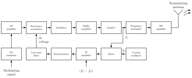
Figure 8.5.7 (Block diagram of FM transmitter): the direct-method chain (AF amplifier → reactance modulator → oscillator → buffer amplifier → limiter → frequency multiplier → RF amplifier → antenna) plus the AFC feedback loop (limiter → mixer with crystal-oscillator reference → IF amplifier → discriminator → low-pass filte …
Drawn by us to help you understand the concept clearly, and verified to make sure it's accurate. For exams, practice from your textbook's own diagram.
The textbook’s Figure 8.5.8 (printed p. 265) shows the pre-emphasis circuit: the audio passes through a capacitor–resistor network whose reactance falls with frequency, so the higher audio frequencies reach the FM modulator with boosted amplitude (the standard 75 time-constant network). The RC values set the corner frequency above which the boost applies — this …
Drawn by us to help you understand the concept clearly, and verified to make sure it's accurate. For exams, practice from your textbook's own diagram.
The textbook’s Figure 8.5.9 (printed p. 265) shows the matching de-emphasis circuit at the receiver: a series resistor feeding a shunt capacitor forms a low-pass RC network with the same 75 time constant, attenuating the highs by exactly the amount pre-emphasis boosted them. Noise picked up in transmission is cut along with the boost, improv …