Transmission lines

A transmission line is a system of conductors that carries electrical energy — as guided electrical waves — from one point to another, for example linking a transmitter or receiver to its antenna. Three types are in common use: the open-wire (two-wire) line, the co-axial cable, and the waveguide.

Equivalent circuit

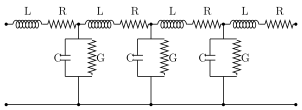
A transmission line is not just a pair of ideal wires; every small length of it has electrical properties distributed along it. Because the wires have length and diameter they possess series resistance R and series inductance L; because the two conductors run close together they form a capacitance C between them; and because the dielectric separating them is not a perfect insulator, a little current leaks across, represented by a shunt conductance G. A line is therefore modelled as a ladder network of series R-L sections with shunt C-G branches (Figure 8.8.1).

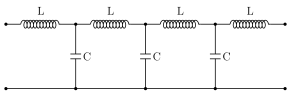
At radio (high) frequencies the inductive reactance $\omega L$ becomes far larger than R, and the capacitive susceptance $\omega C$ far larger than G, so R and G may be neglected. The line then reduces to a simple LC ladder (Figure 8.8.2), which is why a low-loss high-frequency line behaves almost like a pure reactive network.

Primary constants

The four primary constants of a transmission line, specified per unit length, are:

• series resistance R — increases roughly with the square root of frequency;
• series inductance L — for a two-wire line $L = \dfrac{\mu}{2}\,\log\!\left(\dfrac{2D}{d}\right)$, where $\mu$ is the permeability, D the spacing between the wires and d the wire diameter;
• shunt capacitance C — for a two-wire line $C \approx \dfrac{\mu\varepsilon}{\log(2D/d)}$, where $\varepsilon$ is the permittivity;
• shunt conductance G — arising from dielectric loss.

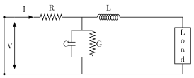
Figure 8.8.3 shows a single section of the line driving a load, with all four primary constants in place.

Secondary constants

The secondary constants of a transmission line are the attenuation constant $\alpha$, the phase-shift constant $\beta$, and the propagation constant $\gamma$, related by

The attenuation constant $\alpha$ measures how the wave amplitude decays along the line, $\beta$ measures the phase change per unit length, and $\gamma$ combines the two. These secondary constants are obtained from the primary constants through the line's per-unit-length series impedance $Z = R + j\omega L$ and shunt admittance $Y = G + j\omega C$. …