Physics · Ch 12 — Electromagnetic Induction
Flux of the Field
Flux of the Field
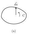
The concept of magnetic flux is central to Faraday's law. Consider a small element of area : by convention, a direction is assigned to this area element such that if the boundary curve is traversed in the sense of a chosen arrow, the area's normal vector points out of the page towards the reader -- exactly the sense in which a right-handed screw would advance if turned in the direction of that arrow (the right-hand screw rule for areas).
If this area element sits in a magnetic field , the flux of through is the scalar quantity , where is the angle between the field direction and the area element's assigned normal direction.
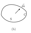
For a FINITE surface , the field need not be uniform across it, so the surface must first be broken into many small area elements , the flux computed through each, and the results summed (integrated) over the whole area: . cannot simply be pulled outside this integral unless it happens to be the same everywhere on S. If, in addition, the field at every point is itself changing with time, the flux becomes an explicit function of time too: . …
Drawn by us to help you understand the concept clearly, and verified to make sure it's accurate. For exams, practice from your textbook's own diagram.
What this figure shows. Shows a small, roughly planar element of area, labelled , bounded by a closed curve drawn with a curved arrow marking a chosen sense of traversal around its boundary (shown as anticlockwise, as viewed by the reader). A short vector arrow is drawn perpendicular to this small area, pointing OUT of the page toward the reader, labelled as the area element's assigned normal direction. The figure fixes the right-handed screw convention linking a boundary-traversal sense to an area-normal direction: curling the right hand's fingers in the direction of the boundary arrow makes the extended thumb point along the assigned normal , exactly as a right-handed scr …
Drawn by us to help you understand the concept clearly, and verified to make sure it's accurate. For exams, practice from your textbook's own diagram.
What this figure shows. Shows a larger, finite curved or flat surface labelled , subdivided by a light grid or a few marked boundary lines into many small patches, one of which is highlighted as a representative small area element (matching Fig. 12.4(a)'s convention) with its own assigned outward normal drawn. The figure illustrates why the magnetic flux through an extended surface cannot simply be written as (field) times (area) in one step when the field is non-uniform over the surface: the surface must first be broken into small elements, the flux computed for each, and the results summed (integrated) over t …