Physics · Ch 12 — Electromagnetic Induction
Induced emf in a Stationary Coil in a Changing Magnetic Field
Induced emf in a Stationary Coil in a Changing Magnetic Field
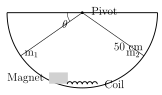
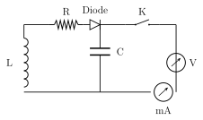
This section studies the complementary case to motional emf: a coil that is itself completely stationary, sitting in a magnetic field whose STRENGTH varies with time. A classic demonstration apparatus makes this concrete: a permanent bar magnet is mounted at the centre of a rigid aluminium arc (radius 50 cm) that can swing freely like a pendulum, threaded through a fixed coil of about 10,000 turns of copper wire so the magnet can pass through the coil as it swings. As the magnet approaches, passes through, and recedes from the coil, the flux linked with the coil rises from a small value to a maximum and falls again, inducing an emf that can be measured by using it to charge a capacitor (through a diode, so only one polarity of pulse charges it) and reading the capacitor's peak voltage.
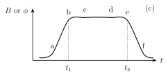
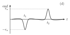
Because the magnet's speed is greatest as it passes through the coil's mean position and much smaller when it is far away, the field (and flux) at the coil changes SLOWLY when the magnet is distant and RAPIDLY as it passes through -- so the induced emf, being proportional to the SLOPE of the flux-vs-time curve, is largest exactly at the two instants (, as the magnet approaches, and , as it leaves) where that slope is steepest, and passes through zero at the very centre of the swing (where flux is momentarily at its maximum and instantaneously constant). Because of Lenz's law's minus sign, the emf pulse is negative while flux is increasing (at ) and positive while it is decreasing (at ) -- so each half-swing of the magnet produces one negative pulse followed by one positive pulse, and the diode charging circuit responds only to the positive pulses, building the capacitor up towards a peak voltage over several oscillations.
Modelling the magnet's oscillation as (amplitude , period T) and the flux as roughly proportional to near the mean position, differentiating gives , which for small angles near the mean position is close to its own maximum value -- so the peak induced emf works out to be directly proportional to the angular amplitude and inversely proportional to the period T of oscillation. …
Drawn by us to help you understand the concept clearly, and verified to make sure it's accurate. For exams, practice from your textbook's own diagram.
What this figure shows. Shows a permanent bar magnet mounted at the centre of a rigid arc-shaped frame (an arc of a semicircle of radius 50 cm, made of aluminium), suspended so the whole arc-and-magnet assembly can swing freely, pendulum-like, within its own plane. A fixed coil of about 10,000 turns of copper wire loops around the arc's path, positioned so that as the arc swings, the magnet passes freely back and forth through the interior of this coil. The figure establishes the physical apparatus used to demonstrate and measure the emf induced in a stationary coil by a magnet whose distance from it varies periodically a …
Drawn by us to help you understand the concept clearly, and verified to make sure it's accurate. For exams, practice from your textbook's own diagram.
What this figure shows. Shows the same fixed coil of Fig. 12.7(a) now connected, across its two terminals, to a small measuring circuit consisting of a capacitor (C) and a diode (D) in series, with a milliammeter (mA) also included in the circuit to monitor charging current. The diode is oriented so current can only flow through it (and hence charge the capacitor) during ONE polarity of the induced emf pulse. The figure shows how the oscillating magnet's induced emf pulses are converted into a measurable, growing DC voltage across the capacitor, which levels off (with the milliammeter reading dropping to zero) once the capacito …
Drawn by us to help you understand the concept clearly, and verified to make sure it's accurate. For exams, practice from your textbook's own diagram.
What this figure shows. A graph with time t on the horizontal axis and the magnetic field B (as measured at the coil, with the magnet at its mean/central swing position) on the vertical axis. The curve is drawn as a single smooth hump (rising from a small baseline value, up to a peak, and back down to the small baseline value again), with a flatter, slightly broadened top portion reflecting the finite physical length of the magnet passing through the coil, and two marked time instants (on the rising, steepening part of the curve, before the peak) and (on the falling, steepening part, after the peak) where the curve's SLOPE is steepest. The figure is purely qualitative (no numeric axis values), us …
Drawn by us to help you understand the concept clearly, and verified to make sure it's accurate. For exams, practice from your textbook's own diagram.
What this figure shows. A companion graph to Fig. 12.7(c), again with time t on the horizontal axis, but now plotting the induced emf e. Corresponding to the steep rising slope of the B-vs-t curve at , this graph shows a pulse of emf that is NEGATIVE (dips below the axis) at ; corresponding to the steep falling slope at , it shows a pulse that is POSITIVE (rises above the axis) at ; the emf is essentially zero both far from the coil (where B changes slowly) and exactly at the peak of the B-curve (where B is momentarily not changing). The figure visually confirms that Lenz's law's minus sign makes the induced emf negative while flux is increasing and p …
Worked out. A coil of N=400 turns, each turn a square of side d=20 cm, sits with its plane perpendicular to an external magnetic field that is switched on and made to rise LINEARLY from 0 to 0.5 T over a time of 0.8 s. Using the flux rule for a stationary coil in a changing field, , with , the induced emf works out to V -- the worked example's own stated result, confirmed by independent recalculation here. …
Worked out. A long solenoid S has 200 turns/cm (i.e. turns/m) and carries a steady current A; its diameter is 3 cm. A smaller coil C, with turns and diameter cm, is wound coaxially so that it sits entirely inside the solenoid's cross-section. The solenoid's current is then steadily reduced to zero over ms. The interior field is T, so the flux linkage with coil C is Wb, and the induced emf is this flux linkage divided by dt: mV -- this own-recalculated value is used since the source page's printed final f …
Worked out. A single conducting loop of area is placed with its plane normal to a uniform magnetic field, which starts at and is uniformly reduced to over a time interval s. Using , the induced emf works out to V. …