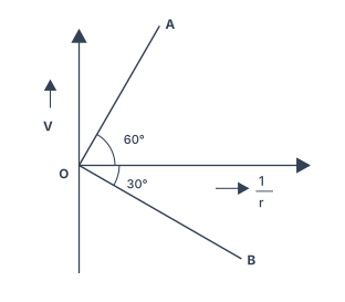
(a)(i) In the figure, OA and OB show the variation of electric potential V at a point due to two point charges

Question

Figure — Figure — CBSE 2026 55/3/1 Q31 — FigureFigure — CBSE 2026 55/3/1 Q31

V

(ii) Two point charges

-2\ \mu\text{C}

and

5\ \mu\text{C}

are placed at

(-30\ \text{cm}, 0)

and

(30\ \text{cm}, 0)

respectively in an external electric field

\vec{E} = \dfrac{A}{x^2}\hat{i}

, where

A = 9\times10^{5}\ \text{Nm}^2\text{C}^{-1}

. Find the electrostatic potential energy of this configuration.

(OR)

(b)(i) Two infinitely long straight wires having linear charge densities

-\lambda

and

3\lambda

are held vertically parallel to each other, a distance

r

apart in free space. Find the nature and magnitude of the force per unit length exerted by one wire on the other.

(ii) A small hollow conducting sphere of radius

r_1

is given a charge

Q

. It is surrounded by a concentric conducting spherical shell of inner radius

r_2

and outer radius

r_3

, carrying charge

-3q

. A point charge

2q

is kept at the centre. Find : (I) the electric flux through a concentric spherical Gaussian surface of radius

x

for

(1)

x < r_1

, and

(2)

r_1 < x < r_2

; (II) the electric field at a point distant

x

from the centre for

(1)

x > r_3

, and

(2)

r_1 < x < r_2

; (III) the surface charge density on the inner surface of

(1) the sphere, and

(2) the shell.

CBSECBSE Class XII Board 2026Subjective· 5mImportance★★★★★

🔒 Locked · start free trial →

You're viewing a preview — the full solution, concept, methods & PYQ mapping are locked.

Start your 14-day free trial to unlock the full solution →

Part (a)Concept understanding — Electric Potential

Electric Potential

The Idea

When you lift a book onto a shelf you do work against gravity, and the book gains gravitational potential energy that depends on where it sits. Electric charges behave the same way in an electric field. Electric potential is the electrical analogue of "height" in a gravitational field: it tells you the potential energy a unit charge would have at a given point.

Formally, the electric potential at a point is the work done in bringing a unit positive charge from infinity to that point, slowly (without giving it kinetic energy), against the electric field.

V = \frac{W}{q_0}

Here $W$ is the work done to move a small test charge $q_0$ from infinity to the point. Because both $W$ and $q_0$ are scalars, electric potential is a scalar quantity — it has magnitude but no direction. Its SI unit is the volt:

1\ \text{V} = 1\ \text{J/C}

Potential Due to a Point Charge

For a single point charge $q$ , the potential at a distance $r$ from it is

V = \frac{1}{4\pi\varepsilon_0}\,\frac{q}{r}

Notice it falls off as $1/r$ , whereas the electric field of a point charge falls off as $1/r^2$ . The potential is taken as zero at infinity, our chosen reference. A positive charge makes the potential around it positive; a negative charge makes it negative.

Potential Difference

Usually we care about the potential difference between two points $A$ and $B$ :

V_A - V_B = \frac{W_{B\to A}}{q_0}

the work per unit charge needed to move a charge from $B$ to $A$ . This is the quantity a voltmeter reads and the "voltage" that drives current in a circuit.

Relation Between Field and Potential

Field and potential are two views of the same thing. The electric field is the negative rate of change of potential with distance:

E = -\frac{dV}{dr}

The minus sign says the field points from high potential toward low potential — a positive charge, left free, rolls "downhill" in potential. Where the potential changes steeply, the field is strong.

Superposition

Because potential is a scalar, the potential due to several charges is just the algebraic sum of their individual potentials — no vectors, no angles:

V = \frac{1}{4\pi\varepsilon_0}\left(\frac{q_1}{r_1} + \frac{q_2}{r_2} + \cdots\right)

This makes potential far easier to compute than the field, which needs vector addition. Once you have $V$ everywhere, you can get the field by differentiating.

Equipotential Surfaces

An equipotential surface is a surface on which the potential has the same value everywhere.

No work is done in moving a charge along an equipotential surface (since $\Delta V = 0$ ).
The electric field is always perpendicular to an equipotential surface. …

Part (b)Concept understanding — Gauss Law

Gauss's Law is a shortcut. Instead of adding up the Coulomb contribution of every charge — a nightmare of vectors and integrals — it lets you read the field straight off the symmetry of a problem. The whole idea rests on one quantity: electric flux.

Flux — field-lines counted through a surface. For a uniform field E crossing a flat area A, the flux is Φ = E·A = EA cosθ, where θ is the angle between the field and the normal to the surface. Picture the field as a bundle of lines; flux is how many pierce the surface. When E is edge-on (θ = 90°) nothing passes through and Φ = 0; when E is ⊥ to the surface (θ = 0) the count is maximal. For a closed surface, Φ is the net number of lines leaving it — lines that enter and exit cancel.

The law itself. Gauss's law states that the net flux out of any closed surface depends only on the charge trapped inside:

Φ = q_enclosed / ε₀.

Two consequences do most of the work. First, only enclosed charge counts — a charge outside sends as many lines in as out, so its net contribution is exactly zero. Second, the surface's shape is irrelevant; move the charge around inside or deform the surface, and Φ never changes.

Why symmetry makes it powerful. By itself Φ = q/ε₀ has E buried in an integral. It becomes a tool only when you pick a Gaussian surface matched to the symmetry — one where E is constant and everywhere either ⊥ to the surface (so Φ = EA) or ∥ to it (contributing nothing). Then E slides out and you solve in one line. This works for exactly three geometries:

1 — Infinite line charge (linear density λ). Use a coaxial cylinder: E = λ / 2πε₀r, falling off as ∝ 1/r.

2 — Infinite sheet (surface density σ). Use a pillbox pierced through the sheet: E = σ / 2ε₀ — uniform and completely independent of distance. The field near a large charged plane simply doesn't weaken as you step back. …

Why this formula?

Gauss's Law: Why It Holds

Gauss's Law is one of the four Maxwell's equations and a cornerstone of electromagnetism. Let's build the understanding from the ground up — not just the formula, but the why.

1. The Core Idea: Flux as "Flow" of Field

Imagine an electric field $\vec{E}$ passing through a small patch of area $dA$ . The electric flux through that patch is:

d\Phi_E = \vec{E} \cdot d\vec{A} = E \, dA \cos\theta

where $\theta$ is the angle between $\vec{E}$ and the outward normal to the surface.

Why this definition?

If $\vec{E}$ is perpendicular to the surface ( $\theta = 0$ ), maximum field "flows through".
If $\vec{E}$ is parallel ( $\theta = 90^\circ$ ), no flux — the field just slides along the surface.

Total flux through a closed surface $S$ is:

\Phi_E = \oint_S \vec{E} \cdot d\vec{A}

2. The Key Insight: Flux Depends Only on Enclosed Charge

Consider a single point charge $+q$ at the centre of a spherical surface of radius $r$ .

By Coulomb's law, at every point on the sphere: $E = \frac{1}{4\pi\varepsilon_0} \frac{q}{r^2}$ , radially outward.
The area vector $d\vec{A}$ is also radially outward.
So $\vec{E} \cdot d\vec{A} = E \, dA$ everywhere.

The total flux:

\Phi_E = \oint E \, dA = E \oint dA = \left( \frac{1}{4\pi\varepsilon_0} \frac{q}{r^2} \right) (4\pi r^2) = \frac{q}{\varepsilon_0}

Notice: The $r^2$ cancels! The flux is independent of the radius.

3. Why Shape Doesn't Matter

Now, what if the surface is not spherical but any closed shape enclosing the charge?

Draw a small cone from the charge to the surface.
The flux through a patch $dA$ at distance $r$ is $d\Phi = \frac{1}{4\pi\varepsilon_0} \frac{q}{r^2} \cos\theta \, dA$ .
But $\frac{\cos\theta \, dA}{r^2}$ is exactly the solid angle $d\Omega$ subtended by $dA$ at the charge.

So $d\Phi = \frac{q}{4\pi\varepsilon_0} d\Omega$ .

Integrating over the entire closed surface: $\oint d\Omega = 4\pi$ (total solid angle around a point).

Hence:

\Phi_E = \frac{q}{4\pi\varepsilon_0} \cdot 4\pi = \frac{q}{\varepsilon_0}

Result: For any closed surface enclosing $q$ , the flux is $\frac{q}{\varepsilon_0}$ .

4. Multiple Charges: Superposition

If there are many charges $q_1, q_2, \dots, q_n$ inside the surface, the total electric field is the vector sum of individual fields:

\vec{E} = \vec{E}_1 + \vec{E}_2 + \dots + \vec{E}_n

Flux is linear: …

Start your 14-day free trial to unlock the full solution →

Part (a): $Q_1>0,\ Q_2<0,\ Q_1/Q_2=-3$ ; total PE in the external field $=20.85\ \text{J}$ . Part (b): $F/L=\dfrac{3\lambda^2}{2\pi\varepsilon_0 r}$ (attractive), plus fluxes, fields and inner-surface densities from Gauss's law.

Part (a) — graph nature and electrostatic PE in an external field

(i) For a point charge, $V=\dfrac{1}{4\pi\varepsilon_0}\dfrac{Q}{r}=kQ\,(1/r)$ ; a $V$ -vs- $1/r$ plot is a line through the origin of slope $kQ$ , as shown in the graph below:

OA has positive slope $\Rightarrow Q_1$ is positive.
OB has negative slope $\Rightarrow Q_2$ is negative. With OA at $60^\circ$ and OB at $30^\circ$ below the axis,

\frac{Q_1}{Q_2}=\frac{\tan60^\circ}{-\tan30^\circ}=\frac{\sqrt3}{-1/\sqrt3}=-3.

(ii) The external field $\vec E=\dfrac{A}{x^2}\hat i$ corresponds to the potential $V(x)=\dfrac{A}{x}$ (since $-dV/dx=A/x^2$ ), with $A=9\times10^{5}\ \text{N m}^2\text{C}^{-1}$ .

The total electrostatic PE of the configuration = energy of each charge in the external field + their mutual interaction energy:

U=q_1V(x_1)+q_2V(x_2)+\frac{1}{4\pi\varepsilon_0}\frac{q_1q_2}{r_{12}}.

With $q_1=-2\times10^{-6}\ \text{C}$ at $x_1=-0.30\ \text{m}$ and $q_2=+5\times10^{-6}\ \text{C}$ at $x_2=+0.30\ \text{m}$ :

q_1V(x_1)=(-2\times10^{-6})\cdot\frac{9\times10^{5}}{-0.30}=+6\ \text{J},

q_2V(x_2)=(+5\times10^{-6})\cdot\frac{9\times10^{5}}{+0.30}=+15\ \text{J}.

Separation $r_{12}=0.60\ \text{m}$ :

$\frac{kq_1q_2}{r_{12}}=\frac{9\times10^{9}\,(-2\times10^{-6})(5\times10^{-6})}{0.60}=\frac{-9\times10^{-2}}{0.60}=-0.15\ \text{J}.$ …

Start your 14-day free trial to unlock the full solution →

Same / Similar Concept — real previous-year questions on the same or a closely similar concept, not this exact question.

Showing the 12 most recent of 81 on this concept.

CBSE 2026Set 55/1/11 markMCQ
$r_1$
›Reveal solutionSolution
When two widely separated conducting spheres are connected by a wire, they reach the same electric potential. Since surface field $E = \frac{kQ}{r^2}$ and potential $V = \frac{kQ}{r}$ , combining these gives $E \propto 1/r$ . Therefore the ratio of surface fields is $E_A/E_B = r_2/r_1$ , which corresponds to option (B).

The key insight here is about what happens when conductors are connected by a wire. Charge flows until both spheres are at the same electric potential — that's the fundamental condition for electrostatic equilibrium in a conductor. Once you grasp that, the rest is just algebra.

Let's think about why potential equality is the right starting point. A conducting wire means the two spheres form a single conductor. In electrostatics, the entire surface of a conductor is an equipotential. So spheres A and B must have the same potential $V$ .

Now, for an isolated conducting sphere of radius $r$ carrying charge $Q$ , the potential at its surface (taking infinity as zero) is:
$V = \frac{1}{4\pi\epsilon_0} \frac{Q}{r}$
And the electric field just outside its surface is:
$E = \frac{1}{4\pi\epsilon_0} \frac{Q}{r^2}$
Notice the relationship: $E = V/r$ . That's a neat shortcut we'll use.

Tip

For any isolated conducting sphere, $E = V/r$ directly. This saves you from carrying the $Q$ through the algebra — just remember it comes from $V = kQ/r$ and $E = kQ/r^2$ .

Let's work through it step by step.

Set potentials equal. Since the wire connects them, $V_A = V_B$ . Using $V = kQ/r$ (where $k = 1/4\pi\epsilon_0$ ):

$k\frac{Q_A}{r_1} = k\frac{Q_B}{r_2}$
Cancel $k$ and rearrange:
$\frac{Q_A}{Q_B} = \frac{r_1}{r_2}$

Write the surface field ratio. For each sphere, $E = kQ/r^2$ . So: $\frac{E_A}{E_B} = \frac{k Q_A / r_1^2}{k Q_B / r_2^2} = \frac{Q_A}{Q_B} \cdot \frac{r_2^2}{r_1^2}$ …
Start your 14-day free trial to see the full solution →
CBSE 2026Set 55/3/11 markMCQ
$m$
›Reveal solutionSolution
Work done by a constant electric field equals force times displacement; since the particle starts from rest, all that work converts to kinetic energy, giving $K = q E_0 x$ .

The heart of this problem is the work-energy theorem: the work done by all forces on a particle equals its change in kinetic energy. When a charged particle moves through an electric field, the field exerts a force that does work, and if the particle starts from rest, every joule of work becomes kinetic energy.

A uniform electric field $\vec{E} = E_0\,\hat{i}$ exerts a force $\vec{F} = q\vec{E}$ on a charge $q$ . This force is constant in magnitude and direction, so the work done is simply force times displacement along the direction of the force.

Step-by-step reasoning

Identify the force on the particle. The electric force on a charge $q$ in field $\vec{E}$ is

$\vec{F} = q\vec{E} = q E_0\,\hat{i}$
The magnitude is $F = q E_0$ , directed along the positive $x$ -axis.

Calculate the work done by this force. The particle moves a distance $x$ along the $x$ -axis, in the same direction as the force. Work done by a constant force is

$W = F \cdot d = q E_0 \cdot x = q E_0 x$

Apply the work-energy theorem. The particle starts from rest, so initial kinetic energy $K_i = 0$ . The work-energy theorem states

$W = \Delta K = K_f - K_i$
Therefore,
$K_f = W = q E_0 x$
The kinetic energy after travelling distance $x$ is simply the work done by the electric field. …
Start your 14-day free trial to see the full solution →
CBSE 2026Set A1 markMCQ
$Q. S.I. unit of electric flux is (A) Vm (B) Vm^2 (C) Jm (D) NC^-1$
›Reveal solutionSolution

Φ = E·A → (V/m)(m²) = V·m.

Electric flux is $\Phi = \vec{E}\cdot\vec{A}$ .

Unit of electric field $E$ = N/C = V/m (volt per metre).

Unit of area $A$ = m².

…

Start your 14-day free trial to see the full solution →
CBSE 2026Set A1 markMCQ
$Q. The surface charge densities on the surface of two conducting spheres of radii r1 and r2 are equal. The ratio of electric field intensities on the surfaces is (A) r1/r2 (B) r1^2/r2^2 (C) r2^2/r1^2 (D) 1 : 1$
›Reveal solutionSolution

Just outside a charged conductor E = σ/ε₀; with equal σ the fields are equal (1:1).

The electric field just outside the surface of a charged conductor is

$E = \frac{\sigma}{\varepsilon_0},$

which depends only on the local surface charge density σ, not on the radius.

…

Start your 14-day free trial to see the full solution →
CBSE 2026Set ANNUAL1 markMCQ
$Q. Electric flux is a$
(a) scalar quantity
(b) vector quantity
(c) scalar or vector quantity
(d) constant quantity
›Reveal solutionSolution

Electric flux is a scalar quantity, even though it is defined using two vectors.

Electric flux through a surface is defined as

$\Phi = \oint \vec{E}\cdot d\vec{A}$

Although $\vec{E}$ (electric field) and $d\vec{A}$ (area vector, normal to the surface element) are both vectors, their dot product $\vec{E}\cdot d\vec{A} = E\,dA\cos\theta$ is a single number (magnitude only, with a sign depending on $\theta$ ) — it …

Start your 14-day free trial to see the full solution →
CBSE 2026Set ANNUAL1 markMCQ
$Q. A charge Q, is enclosed by a Gaussian spherical surface of radius R. If the radius is doubled, then the outward electric flux will$
(a) decrease to half
(b) increase two times
(c) remain unchanged
(d) increase four times
›Reveal solutionSolution

Gauss's law: flux through any closed surface = Q_enclosed / epsilon_0, and this does NOT depend on the surface's size or shape.

Gauss's law states that for any closed (Gaussian) surface,

flux (phi) = Q_enclosed / epsilon_0

Here the same charge Q sits at the centre of the sphere both before and after the radius is doubled - the enclosed charge Q_enclosed is unchanged. Since flux depends ONLY on Q_enclosed and the permittivity of free space epsilon_0 (both unchanged here), the flux does not change even though the surface area (4piR^2) has increased fourfold. Doubling R spreads the same total flux over 4 ti …

Start your 14-day free trial to see the full solution →
CBSE 2026Set ANNUAL1 markMCQ
$Q. SI unit of electric potential is:$
(a) Ohm
(b) Volt
(c) Coulomb
(d) Ampere
›Reveal solutionSolution

Electric potential is defined as work done per unit charge, so its SI unit is the Volt.

Electric potential at a point is $V = \dfrac{W}{q}$ , i.e. the work done in bringing a unit positive charge from infinity to that point. Since work is measured in joules (J) and charge in coulombs (C), the unit o …

Start your 14-day free trial to see the full solution →
CBSE 2026Set ANNUAL1 markMCQ
$Q. [Case study, continued] The charges q1 and q2 produce a potential, which at any point P will be$
(a) V1,2 = 1/(4πε₀) × (q1/r1P² + q2/r2P²)
(b) V1,2 = 1/(4πε₀) × (q1/r1P + q2/r2P)
(c) V1,2 = 1/(4πε₀) × (q1/r1P - q2/r2P)
(d) V1,2 = 1/(4πε₀) × (2q1/r1P + 3q2/r2P)
›Reveal solutionSolution

The potential due to a group of point charges at any point is just the plain algebraic (scalar) sum of the potentials each charge produces there — the superposition principle for potential.

Electric potential obeys the superposition principle: the total potential at any point due to several charges equals the SCALAR sum (not vector sum, since potential is a scalar) of the potentials due to each individual charge, each given by $V = \dfrac{1}{4\pi\varepsilon_0}\dfrac{q}{r}$ (distance to the first power).

For two charges $q_1$ (at distance $r_{1P}$ from P) and $q_2$ (at distance $r_{2P}$ from P):

$V_{1,2} = \frac{1}{4\pi\varepsilon_0}\left(\frac{q_1}{r_{1P}} + \frac{q_2}{r_{2P}}\right)$

…

Start your 14-day free trial to see the full solution →
CBSE 2026Set ANNUAL1 markMCQ
$R$
(a) increases as $r$ increases for $r<R$ and for $r>R$
(b) is zero as $r$ increases for $r<R$ and decreases as $r$ increases for $r>R$
(c) is zero as $r$ increases for $r<R$ and increases as $r$ increases for $r>R$
(d) decreases as $r$ increases for $r<R$ and for $r>R$
›Reveal solutionSolution

A charged conducting (hollow metal) sphere carries all its charge on the outer surface. Gauss's law gives $E=0$ inside and $E\propto 1/r^2$ (decreasing) outside.

Setting up Gauss's law

For a hollow, uniformly charged conducting sphere of radius $R$ and total charge $Q$ , all the charge resides on the outer surface (a fundamental property of conductors in electrostatic equilibrium — free charges repel each other and move to the surface where the electric field inside the conducting material is zero).

Take a concentric spherical Gaussian surface of radius $r$ .

Case 1: $r<R$ (inside the shell)

The Gaussian surface of radius $r$ encloses no charge, because all the charge $Q$ lies on the surface at radius $R>r$ .

$\oint \vec E\cdot d\vec A = \frac{Q_{\text{enc}}}{\varepsilon_0} = 0 \implies E=0$

This is true for every $r<R$ — the field is zero throughout the interior, it does not "increase" or "decrease," it is simply zero.

Case 2: $r>R$ (outside the shell)

Now the Gaussian surface encloses the entire charge $Q$ . By spherical symmetry, $\vec E$ is radial and has the same magnitude everywhere on the Gaussian sphere, so

…

Start your 14-day free trial to see the full solution →
CBSE 2026Set ANNUAL1 markMCQ
$Q. The standard potential of earth is :$
(a) Zero
(b) Infinite
(c) One
(d) None of the above
›Reveal solutionSolution

The Earth is the chosen reference for potential, so its standard potential is taken as zero.

Electric potential is always measured relative to some reference. Because the Earth is a very large conductor whose potential is practically unaffected by adding or removing charge, it is universally chosen as the reference (zero) level of potential.

…

Start your 14-day free trial to see the full solution →
CBSE 2026Set ANNUAL1 mark
$Q. Match the Column A with Column B and write the correct pair. Column A: Electric flux. Column B:$
(i) μ₀nI,
(ii) Volt × second,
(iii) μ₀nI/2,
(iv) Volt × meter,
(v) Volt × meter⁻¹,
(vi) Volt.
›Reveal solutionSolution

Electric flux φ_E = E·A; unit = (V/m)(m²) = V·m, option (iv).

Electric flux through a surface is φ_E = E·A (for a uniform field perpendicular to area A). The SI unit of electric field E is volt per metre (V/m) = N/C, and area is in m². Therefore the unit of electric flux is

…

Start your 14-day free trial to see the full solution →
CBSE 2026Set ANNUAL1 mark
$Q. Match the Column A with Column B and write the correct pair. Column A: Potential gradient. Column B:$
(i) μ₀nI,
(ii) Volt × second,
(iii) μ₀nI/2,
(iv) Volt × meter,
(v) Volt × meter⁻¹,
(vi) Volt.
›Reveal solutionSolution

Potential gradient dV/dx has unit V/m = Volt × metre⁻¹, option (v).

The potential gradient is the rate of change of electric potential with distance, dV/dx. Its SI unit is volt per metre (V/m), i.e. Volt × metre⁻¹. In magnitude it equals th …

Start your 14-day free trial to see the full solution →

Part (a)Concept understanding — Electric Potential

Electric Potential

The Idea

Potential Due to a Point Charge

Potential Difference

Relation Between Field and Potential

Superposition

Equipotential Surfaces

Part (b)Concept understanding — Gauss Law

Why this formula?

Gauss's Law: Why It Holds

1. The Core Idea: Flux as "Flow" of Field

2. The Key Insight: Flux Depends Only on Enclosed Charge

3. Why Shape Doesn't Matter

4. Multiple Charges: Superposition

Potential, energy in an external field, and Gauss's law

Part (a) — graph nature + energy of two charges

Part (a) — graph nature and electrostatic PE in an external field

Step-by-step reasoning

Part (a) — graph nature and electrostatic PE in an external field

🎓Unlock everything free for 14 days

Unlock everything free for 14 days