Physics · Ch 8 — Electrostatics

Electric Potential due to a Point Charge

8.4.1

Electric Potential due to a Point Charge

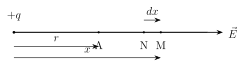
Let a point charge $+q$ sit at the origin O, and let A be a field point at distance $r$ from it. To find the potential at A -- by definition, the work needed to bring a unit positive test charge from infinity to A -- choose the most convenient path: a straight line running from infinity, through an intermediate point M at distance $x$ from O, all the way in to A at $x=r$ .

At M, the outward Coulomb force on the unit test charge is $F=\dfrac{1}{4\pi\epsilon_0}\dfrac{q}{x^2}$ . For a small further inward step $dx$ (moving from a point N farther out toward M, i.e. toward O), the work done is $dW=-F\,dx$ , the minus sign appearing because the displacement is directed opposite to the outward-pointing force. Integrating this from $x=\infty$ down to $x=r$ gives the total work: $W=\displaystyle\int_{\infty}^{r}-F\,dx=\dfrac{1}{4\pi\epsilon_0}\dfrac{q}{r}$ . By the very definition of potential, this work IS the potential at A: $V=\dfrac{1}{4\pi\epsilon_0}\dfrac{q}{r}$ .

Several important features follow directly from this single formula. A POSITIVE source charge always produces a positive potential everywhere around it, and a NEGATIVE source charge always produces a negative potential -- unlike the field, whose sign convention is about direction, the sign of $V$ is a genuine, physically meaningful positive-or-negative NUMBER. As $r\to\infty$ , $V\to0$ , consistent with the zero-at-infinity convention chosen in section 8.3. Since $V$ depends on $r$ ALONE, with no dependence at all on direction, the potential of a single point charge is spherically SYMMETRIC -- every sphere of fixed radius around the charge is at one single, common potential value (developed fully as the idea of an "equipotential surface" in section 8.5). …

Figure 8.6Fig. 8.6: Electric potential due to a point charge

Fig. 8.6 — Fig. 8.6: Electric potential due to a point charge

Drawn by us to help you understand the concept clearly, and verified to make sure it's accurate. For exams, practice from your textbook's own diagram.

What this figure shows. A point charge $+q$ located at point O, with a field point A at distance $r$ from it, and an intermediate point M at distance $x$ from O lying on the straight line from O out to infinity through A. A small further displacement $dx$ from M toward a neighbouring point N (still further from O) is marked, with the outward Coulomb force on a unit positive test charge at M drawn as an arrow pointing away from O along OM extended -- the exact geometric set-up used to integrate $dW=-Fdx$ from infinity down to $r$ and arrive at $V …

Figure 8.7Fig. 8.7: Variation of electric field and potential with distance

Fig. 8.7 — Fig. 8.7: Variation of electric field and potential with distance

Drawn by us to help you understand the concept clearly, and verified to make sure it's accurate. For exams, practice from your textbook's own diagram.

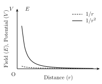
What this figure shows. A graph with two curves plotted on the same distance ( $r$ ) axis: one curve for electric field $E$ , following an inverse-square ( $E\propto1/r^2$ ) shape -- very steep near small $r$ , falling rapidly and flattening toward (but never reaching) zero as $r$ grows large; and a second curve for potential $V$ , following an inverse-first-power ( $V\propto1/r$ ) shape, which is also decreasing but visibly falls off MORE GENTLY than the $E$ curve at the same large- $r$ values, so the two curves are close together near the charge but the $V$ curve sits noticeably above the $E$ curve at greater distances -- the graphical statement that $V$ decreas …

Misc Ex.6Example 8.6: Potential at the centre of a uniformly charged ring

Worked out. A wire bent into a circle of radius $R=10\,\text{cm}=10^{-1}$ m carries a total charge $q=250\,\mu C=250\times10^{-6}$ C spread uniformly on it. Since every point on the wire is the SAME distance $R$ from the centre, the potential there is found exactly as for a single point charge of the same total magnitude at that distance: $V=\dfrac{1}{4\pi\epsilon_0}\dfrac{q}{R}=9\times10^9\times\dfrac{250\times10^{-6}}{10^{-1}}=2.25\times10^7$ volt -- illustrating that potential, being a scalar that simply adds up (unlike the vector field), lets many equidistant charge elements be summed as if t …

Start your 14-day free trial to unlock the full solution →

← Previous · 8.4Electric Potential due to a Point Charge, a Dipole and a System of Charges Next · 8.4.2 →Electric Potential due to an Electric Dipole