Electric Potential due to an Electric Dipole

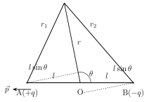
Place the origin at the centre O of an electric dipole: charge $-q$ at point A and $+q$ at point B, separated by $2l$, with dipole moment $\vec{p}=q(2\vec{l})$ pointing from $-q$ to $+q$. Let C be a field point at distance $r$ from O, at angle $\theta$ to the dipole axis, with $r_1$ its distance from the $-q$ charge and $r_2$ its distance from the $+q$ charge.

By the ordinary superposition of two point-charge potentials (section 8.4.1 applied twice), $V_C=\dfrac{1}{4\pi\epsilon_0}\left(\dfrac{q}{r_2}-\dfrac{q}{r_1}\right)$. Using the cosine rule in the triangle formed by O, C and each charge, $r_1^2=r^2+l^2+2rl\cos\theta$ and $r_2^2=r^2+l^2-2rl\cos\theta$. For a SHORT dipole viewed from far away ($r\gg l$), the $l^2$ term can be dropped and a first-order binomial expansion, $(1+x)^n\approx1+nx$ for small $x$, applied to each of $1/r_1$ and $1/r_2$. Carrying this through and keeping only the leading term in $l/r$ collapses the whole expression down to the compact result $V_C=\dfrac{1}{4\pi\epsilon_0}\dfrac{p\cos\theta}{r^2}=\dfrac{1}{4\pi\epsilon_0}\dfrac{\vec{p}\cdot\hat{r}}{r^2}$ -- notice this falls off as $1/r^2$, one power FASTER than a single point charge's $1/r$ potential, because at large distances the dipole's two opposite charges' potentials nearly cancel, and only the small residual imbalance (proportional to $p=q\cdot2l$) survives. …