Reference Circle Method

Sections 5.4-5.6 built up the mathematics of linear S.H.M. from the differential equation onward. This section takes a completely different, purely GEOMETRIC route to the exact same equations, by relating linear S.H.M. to uniform circular motion (U.C.M.) -- a connection so useful that $\omega$ is called the "angular frequency" of an S.H.M. precisely because of it.

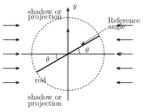
Picture a thin rod, pivoted at its centre, rotating uniformly in a vertical circle that lies in the x-y plane (Fig. 5.3). If this rod is illuminated from one side by a linear light source oriented parallel to the rod itself, its SHADOW falls on the y-axis. As the rod rotates around and around at constant angular speed, the tip of this shadow does NOT move at constant speed along the y-axis -- instead, it can be seen oscillating back and forth about the origin. The claim of this section is that this shadow motion is not merely "oscillation-like" -- it is EXACTLY a linear S.H.M., and working out its equations is a matter of straightforward geometry (projection) rather than solving a differential equation.

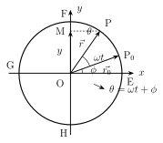
Set up the geometry precisely (Fig. 5.4): let a particle P perform anticlockwise uniform circular motion of radius r about a centre O, with angular velocity $\omega$. Angular positions are measured from a fixed reference direction OX (so a particle at E, on OX itself, is at angular position zero; at F, 90 degrees further round, at angular position $\pi/2$; at G, 180 degrees round, at angular position $\pi$; and so on). Suppose at time t = 0 the particle is at some position $P_0$, at reference angle $\phi$ from OX. By time t, it has swept out a further angle $\omega t$, so its total reference angle (the angle OP makes with OX) at time t is $(\omega t + \phi)$.

Choose a reference diameter -- say, the diameter FH lying along the y-axis -- and let M be the foot of the perpendicular dropped from P onto this diameter, so OM is the PROJECTION of the particle's position vector OP onto the chosen diameter. From the right-angled geometry, the length OM (call it y, the projected displacement) is

This is EXACTLY the equation of a linear S.H.M. of amplitude r (compare directly with Eq. 5.12, $x = A\sin(\omega t+\phi)$, with r playing the role of A). The angular velocity $\omega$ of the reference circular motion is thus revealed as exactly the same $\omega$ we have been calling the "angular frequency" of the S.H.M. -- the projection of the U.C.M.'s angular velocity becomes the S.H.M.'s angular frequency.

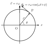
The same projection trick works for velocity and acceleration too. In the U.C.M., the particle's instantaneous (tangential) velocity has magnitude $r\omega$, directed tangent to the circle at P (Fig. 5.5); its projection onto the reference diameter works out (again by the right-angled geometry, now involving the angle between the tangential-velocity direction and the diameter) to

which matches exactly the S.H.M. velocity expression from section 5.5. Similarly, the U.C.M. particle's centripetal (radial) acceleration, of magnitude $r\omega^2$ and always directed towards the centre O, projects onto the reference diameter as …