Ampere's Law

The Biot-Savart law (Section 10.10) is completely general -- it can, in principle, be used to find the magnetic field of ANY current distribution, however complicated -- but, as the sometimes-lengthy integrations of Sections 10.10.1 through 10.13 show, DIRECTLY carrying out that integration can be a genuinely laborious business, even for fairly simple, highly symmetric current shapes. Recall the exactly parallel situation in electrostatics: Coulomb's law is likewise completely general, but Gauss's law offers a dramatic shortcut whenever the CHARGE distribution has enough symmetry (spherical, cylindrical, or planar). Ampere's law is the magnetostatic counterpart of exactly that idea, offering the same kind of shortcut whenever the CURRENT distribution is sufficiently symmetric.

Ampere's circuital law states that

where the integral (denoted by the circle through the integral sign) is taken all the way around any closed path, called an "Amperian loop," and $I$ on the right-hand side is the NET current actually encircled (enclosed) by that particular loop -- currents lying entirely OUTSIDE the chosen loop contribute nothing to the integral, since their field's tangential (along-the-loop) component integrates to exactly zero over a full loop that does not enclose them.

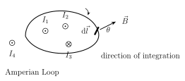
To apply this law correctly, a definite sign convention is needed for currents that might flow in different directions relative to the chosen loop. The convention (Fig. 10.22) uses the same right-hand curl idea seen throughout the chapter: curl the fingers of the right hand along the SENSE OF INTEGRATION chosen for traversing the Amperian loop; a current flowing along the direction the outstretched THUMB then points is counted as POSITIVE, and a current flowing in the opposite direction is counted as NEGATIVE. Currents lying outside the loop are simply not counted (their net contribution to the integral cancels regardless of sign, as noted above). With this convention, for a loop encircling currents $I_1$, $I_2$ (out of the page, hence positive by the chosen sense) and $I_3$ (into the page, hence negative), with a fourth current $I_4$ lying outside the loop altogether,

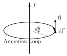
As an immediate demonstration of the power of this law, apply it to re-derive the field of a long straight wire (already found the "hard way," by direct Biot-Savart integration, in Section 10.10.1). Choose a CIRCULAR Amperian loop of radius $r$, centred on and coaxial with the wire (Fig. 10.23). By the wire's cylindrical symmetry, $B$ has the same magnitude everywhere on this loop, and is directed exactly TANGENT to the circle at every point -- exactly parallel to $d\vec{l}$ everywhere along this particular choice of loop, so $\vec{B}\cdot d\vec{l}=B\,dl$ (no cosine factor needed) at every point. Ampere's law then gives, almost by inspection,

$\oint B\,dl = B\oint dl = B(2\pi r) = \mu_0 I \quad\Rightarrow\quad B = \frac{\mu_0 I}{2\pi r},$ …