Physics · Ch 10 — Magnetic Fields due to Electric Current
Magnetic Field due to a Current: Biot-Savart Law
Magnetic Field due to a Current: Biot-Savart Law
Sections 10.1 through 10.9 dealt entirely with the FIRST half of this chapter's subject: given a magnetic field, what force (and torque) does it exert on a moving charge or a current? The remaining sections turn to the SECOND half: given a current, what magnetic field does IT produce? The qualitative answer -- a current-carrying wire is surrounded by a magnetic field circling around it, in the sense given by the right-hand thumb rule -- was already stated back in Section 10.1. What has been missing so far is a way to calculate this field QUANTITATIVELY, for a current of any given strength and a wire of any given shape, at any point in space.
That quantitative tool is the Biot-Savart law, an experimentally-deduced result (much as Coulomb's law was, in electrostatics) for the differential magnetic field produced at a point P by a small current element (Fig. 10.15). If is the position vector from the current element to the point P (of magnitude ), and is the angle between and , the MAGNITUDE of the differential field is
where T.m/A is a fundamental constant called the permeability of free space (or the "permeability constant"), fixing the overall strength of magnetic effects in vacuum, exactly as (or the constant ) fixes the strength of electrostatic effects in Coulomb's law. Notice that this is, at its core, still an INVERSE-SQUARE law -- the field falls off as -- exactly the same power-law dependence as Coulomb's law for a point charge, even though the "source" here is a moving-charge current element rather than a static point charge.
The DIRECTION of is fixed by the vector cross product (where is the unit vector along ), giving the full vector form of the Biot-Savart law:
…
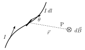
Drawn by us to help you understand the concept clearly, and verified to make sure it's accurate. For exams, practice from your textbook's own diagram.
What this figure shows. A current-carrying wire of arbitrary (curved) shape carries a steady current I. A small differential length element dl is marked at one point along the wire, with the current in this element flowing in the direction of the length vector . A separate point P is marked away from the wire, with a vector drawn FROM the current element dl TO the point P, of magnitude r. A cross symbol () is drawn at P, indicating that the differential magnetic field produced there by this one current element is directed INTO the plane of the paper -- this is the general Biot-Savart-law setup that every specific field calculation in the rest of the chapter (straight wire, arc, loop) is …