Physics · Ch 10 — Magnetic Fields due to Electric Current
Magnetic Field due to a Long Straight Wire
Magnetic Field due to a Long Straight Wire
As the first, and most basic, application of the Biot-Savart law, consider a long straight wire carrying current , and a point P at perpendicular distance from the wire (Fig. 10.16). Using the right-hand thumb rule (already familiar from Section 10.1), the field at P is directed into the plane of the paper (for the current direction shown), so only its MAGNITUDE needs to be worked out by integration.
Take a current element of infinitesimal length , situated a distance from P, making angle with the line joining it to P. By the Biot-Savart law, this element contributes a differential field of magnitude
The total field at P is found by integrating this contribution over the ENTIRE length of the wire -- conveniently split into the upper half (integrated from the point closest to P out to infinity) and the lower half (by symmetry, contributing an identical magnitude, in the same direction, as the upper half), so that
Using the right-triangle geometry relating the perpendicular distance , the along-wire distance (measured from the foot of the perpendicular from P), and , together with , this integral can be carried out explicitly (most conveniently via the standard trigonometric substitution , , with the limits and ), giving, for the field due to a SEMI-INFINITE wire (one half only, from the foot of the perpendicular out to infinity in one direction),
Adding the equal contribution from the other (semi-infinite) half of an INFINITELY long wire doubles this result, giving the standard, widely-used formula for the field due to a long straight wire, at perpendicular distance :
…
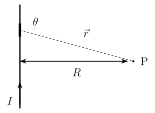
Drawn by us to help you understand the concept clearly, and verified to make sure it's accurate. For exams, practice from your textbook's own diagram.
What this figure shows. A long straight current-carrying wire of length l lies along a vertical line, carrying current I. A point P is marked at a perpendicular distance R from the wire (the perpendicular foot on the wire is marked, with R drawn as the horizontal distance from that foot to P). A current element on the wire is joined to P by a vector r, making an angle with the wire's own length direction. A symbol () at P indicates that the differential field produced there by this element is directed INTO the plane of the paper -- setting up exactly the geometry (r, R, l, all related by the right-triangle formed by the wire, the perpendicular R, and the line r to P) used in …