Physics · Ch 10 — Magnetic Fields due to Electric Current

Arbitrarily Shaped Wire

10.5.2

Arbitrarily Shaped Wire

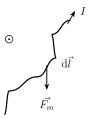
The straight-wire result of Section 10.5.1, $\vec{F}_m=I\vec{L}\times\vec{B}$ , applies directly only when the current-carrying conductor is itself perfectly straight. Real circuits, however, very often involve wires bent into all kinds of shapes -- loops, coils, arcs -- so it is essential to extend the result to a wire of ARBITRARY (possibly curved) shape (Fig. 10.9). The key idea, used repeatedly throughout this chapter (and, more generally, throughout electromagnetism), is to break the curved wire up into a very large number of tiny, effectively-straight segments, each so short that it can be treated as a straight "current element" $Id\vec{l}$ , apply the already-known straight-wire result to each such infinitesimal element, and then sum (integrate) the contributions of every element along the whole wire.

For a current element of infinitesimal length $d\vec{l}$ , carrying current $I$ , sitting in a magnetic field $\vec{B}$ (here specifically taken perpendicular to the plane of the wire, coming out of the page, for concreteness), the differential force it experiences is, directly from the straight-wire law applied to this tiny segment,

d\vec{F}_m = I\,d\vec{l}\times\vec{B}.

The TOTAL force on the entire wire is then obtained by integrating this differential force over the whole length of the wire:

\vec{F}_m = \int d\vec{F}_m = I\int d\vec{l}\times\vec{B}.

In the important special case where $\vec{B}$ is UNIFORM over the entire wire (the same at every point along it, which is a very common practical situation), $\vec{B}$ can be pulled entirely outside the integral, since it no longer varies from one current element to the next:

$\vec{F}_m = I\left(\int d\vec{l}\right)\times\vec{B}.$ …

Figure 10.9Fig. 10.9: Wire with arbitrary shape

Fig. 10.9 — Fig. 10.9: Wire with arbitrary shape

Drawn by us to help you understand the concept clearly, and verified to make sure it's accurate. For exams, practice from your textbook's own diagram.

What this figure shows. A current-carrying wire is drawn bent into an irregular, arbitrary curved shape (not straight), carrying a steady current I along its length. A small representative element of the wire, of infinitesimal length dl, is highlighted somewhere along the curve, with a short arrow drawn tangent to the wire at that point representing the vector $d\vec{l}$ (in the direction of the local current flow). The figure's purpose is purely geometric: it establishes that ANY shaped wire can be broken up into many such small, effectively-straight current elements $Id\vec{l}$ , each of which can be treated by the straight-wire force law of …

Misc Ex.10.2Sign of the charge and momentum of a particle from its trajectory in a field strip

Worked out. A particle of charge q follows a curved trajectory through a strip-shaped region bounded by two parallel lines pp' (a uniform magnetic field $\vec{B}$ , directed out of the plane of the paper, exists only within this strip); the particle enters moving in the positive x direction and is observed to curve UPWARD as it crosses the strip. Since $\vec{v}\times\vec{B}$ for the entering velocity works out to the negative y direction, but the observed force (and hence curving) is in the positive y direction, the charge must be NEGATIVE (only a negative charge flips $q\vec{v}\times\vec{B}$ into the opposite, observed, sense). Using the chord geometry of the circular arc traced inside the strip (of width S, with the particle deflected upward by a further distance L by the time it exits, so that $(R-S)^2+L^2=R^2$ for the circle's radius R), the example solves this geometric relation for $R=\frac{S^2+L^2}{2S}$ , and then substitutes into the cyclotron relation $p=qBR$ to express the particle's momentum entir …

Start your 14-day free trial to unlock the full solution →

← Previous · 10.5.1Straight Wire Next · 10.6 →Force on a Closed Circuit in a Magnetic Field B